Climate sensitivity and feedback#
Radiative forcing#
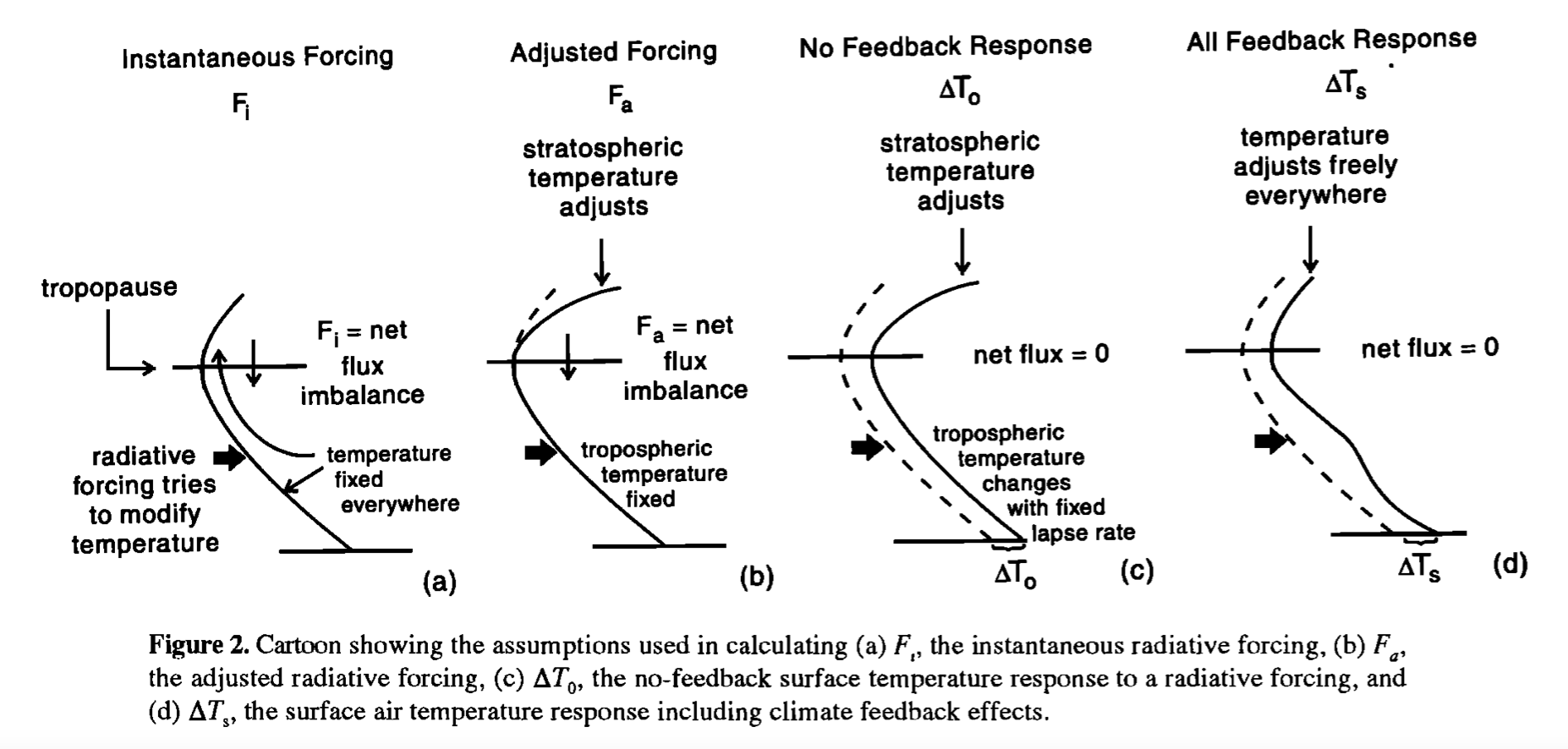
We start with the radiative forcing in a RCE model. Recall that the instantaneous radiative forcing is the quick change in the TOA energy budget before the climate system begins to adjust.
If we consider the forcing as doubling CO2, we could write the radiative forcing as:
What is happening after we add more CO2 in the atmosphere?
The atmosphere is less efficient at radiating energy away to space (reducing emissivity, right?).
OLR will decrease
The climate system will begin gaining energy.
Now let’s build a RCE model and analyze its radiative forcing.
#  This code is used just to create the skew-T plot of global, annual mean air temperature
%matplotlib inline
import numpy as np
import matplotlib.pyplot as plt
import xarray as xr
from metpy.plots import SkewT
import climlab

#plt.style.use('dark_background')

#  This code is used just to create the skew-T plot of global, annual mean air temperature
#ncep_url = "http://www.esrl.noaa.gov/psd/thredds/dodsC/Datasets/ncep.reanalysis.derived/"
ncep_url = "/Users/yuchiaol_ntuas/Desktop/ebooks/data/"
#time_coder = xr.coders.CFDatetimeCoder(use_cftime=True)
ncep_air = xr.open_dataset( ncep_url + "air.mon.1981-2010.ltm.nc", use_cftime=True)
#  Take global, annual average
coslat = np.cos(np.deg2rad(ncep_air.lat))
weight = coslat / coslat.mean(dim='lat')
Tglobal = (ncep_air.air * weight).mean(dim=('lat','lon','time'))

print(Tglobal)

#  Resuable function to plot the temperature data on a Skew-T chart
def make_skewT():
    fig = plt.figure(figsize=(9, 9))
    skew = SkewT(fig, rotation=30)
    skew.plot(Tglobal.level, Tglobal, color='black', linestyle='-', linewidth=2, label='Observations')
    skew.ax.set_ylim(1050, 10)
    skew.ax.set_xlim(-90, 45)
    # Add the relevant special lines
    skew.plot_dry_adiabats(linewidth=0.5)
    skew.plot_moist_adiabats(linewidth=0.5)
    #skew.plot_mixing_lines()
    skew.ax.legend()
    skew.ax.set_xlabel('Temperature (degC)', fontsize=14)
    skew.ax.set_ylabel('Pressure (hPa)', fontsize=14)
    return skew

#  and a function to add extra profiles to this chart
def add_profile(skew, model, linestyle='-', color=None):
    line = skew.plot(model.lev, model.Tatm - climlab.constants.tempCtoK,
             label=model.name, linewidth=2)[0]
    skew.plot(1000, model.Ts - climlab.constants.tempCtoK, 'o',
              markersize=8, color=line.get_color())
    skew.ax.legend()
<xarray.DataArray (level: 17)> Size: 68B
array([ 15.179084  ,  11.207003  ,   7.8383274 ,   0.21994135,
        -6.4483433 , -14.888848  , -25.570469  , -39.36969   ,
       -46.797905  , -53.652245  , -60.56356   , -67.006065  ,
       -65.53293   , -61.48664   , -55.853584  , -51.593952  ,
       -43.21999   ], dtype=float32)
Coordinates:
  * level    (level) float32 68B 1e+03 925.0 850.0 700.0 ... 50.0 30.0 20.0 10.0
# Get the water vapor data from CESM output
#cesm_data_path = "http://thredds.atmos.albany.edu:8080/thredds/dodsC/CESMA/"
cesm_data_path = "/Users/yuchiaol_ntuas/Desktop/ebooks/data/"
atm_control = xr.open_dataset(cesm_data_path + "cpl_1850_f19.cam.h0.nc")
# Take global, annual average of the specific humidity
weight_factor = atm_control.gw / atm_control.gw.mean(dim='lat')
Qglobal = (atm_control.Q * weight_factor).mean(dim=('lat','lon','time'))

#  Make a model on same vertical domain as the GCM
mystate = climlab.column_state(lev=Qglobal.lev, water_depth=2.5)
#  Build the radiation model -- just like we already did
rad = climlab.radiation.RRTMG(name='Radiation',
                              state=mystate,
                              specific_humidity=Qglobal.values,
                              timestep = climlab.constants.seconds_per_day,
                              albedo = 0.25,  # surface albedo, tuned to give reasonable ASR for reference cloud-free model
                             )
#  Now create the convection model
conv = climlab.convection.ConvectiveAdjustment(name='Convection',
                                               state=mystate,
                                               adj_lapse_rate=6.5,
                                               timestep=rad.timestep,
                                              )
#  Here is where we build the model by coupling together the two components
rcm = climlab.couple([rad, conv], name='Radiative-Convective Model')

print(rcm)

print(rcm.subprocess['Radiation'].absorber_vmr['CO2'])

print(rcm.integrate_years(5))

print(rcm.ASR - rcm.OLR)
climlab Process of type <class 'climlab.process.time_dependent_process.TimeDependentProcess'>.
State variables and domain shapes:
  Ts: (1,)
  Tatm: (26,)
The subprocess tree:
Radiative-Convective Model: <class 'climlab.process.time_dependent_process.TimeDependentProcess'>
   Radiation: <class 'climlab.radiation.rrtm.rrtmg.RRTMG'>
      SW: <class 'climlab.radiation.rrtm.rrtmg_sw.RRTMG_SW'>
      LW: <class 'climlab.radiation.rrtm.rrtmg_lw.RRTMG_LW'>
   Convection: <class 'climlab.convection.convadj.ConvectiveAdjustment'>

0.000348
Integrating for 1826 steps, 1826.2110000000002 days, or 5 years.
Total elapsed time is 4.999422301147019 years.
None
[-3.3651304e-11]
Now we make another RCE model with CO2 doubled!
# Make an exact clone with same temperatures
rcm_2xCO2 = climlab.process_like(rcm)
rcm_2xCO2.name = 'Radiative-Convective Model (2xCO2 initial)'

#  Check to see that we indeed have the same CO2 amount
print(rcm_2xCO2.subprocess['Radiation'].absorber_vmr['CO2'])

#  Now double it!
rcm_2xCO2.subprocess['Radiation'].absorber_vmr['CO2'] *= 2

print(rcm_2xCO2.subprocess['Radiation'].absorber_vmr['CO2'])
0.000348
0.000696
Let’s quickly chech the instantaneous radiative forcing:
rcm_2xCO2.compute_diagnostics()

print(rcm_2xCO2.ASR - rcm.ASR)

print(rcm_2xCO2.OLR - rcm.OLR)

DeltaR_instant = (rcm_2xCO2.ASR - rcm_2xCO2.OLR) - (rcm.ASR - rcm.OLR)

print(DeltaR_instant)
[0.06274162]
[-2.11458541]
[2.17732704]
What is the instantaneous radiative forcing in our two/three-layer model?
Now we briefly calculate the adjusted radiative forcing. Recall that the adjusted radiative forcing is that the stratosphere is adjusted while the troposphere does not.
# print out troposphere
print(rcm.lev[13:])

rcm_2xCO2_strat = climlab.process_like(rcm_2xCO2)
rcm_2xCO2_strat.name = 'Radiative-Convective Model (2xCO2 stratosphere-adjusted)'
for n in range(1000):
    rcm_2xCO2_strat.step_forward()
# hold tropospheric and surface temperatures fixed
    rcm_2xCO2_strat.Tatm[13:] = rcm.Tatm[13:]
    rcm_2xCO2_strat.Ts[:] = rcm.Ts[:]

DeltaR = (rcm_2xCO2_strat.ASR - rcm_2xCO2_strat.OLR) - (rcm.ASR - rcm.OLR)
print(DeltaR)
[226.513265 266.481155 313.501265 368.81798  433.895225 510.455255
 600.5242   696.79629  787.70206  867.16076  929.648875 970.55483
 992.5561  ]
[4.28837377]
Radiative forcing gives us some insights about how the changes of forcing could tranfer energy to the system, and temperature might change. But not the final temperature reaching equilibrium.
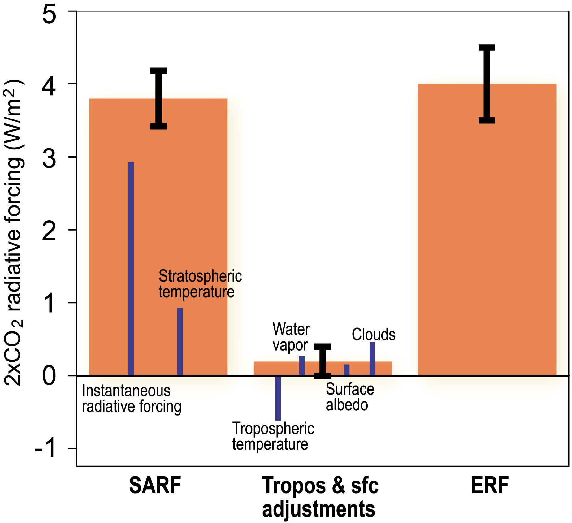
Sherwood et al. (2020) summarize the radiative forcing:
Equilibrium climate sensitivity (ECS) without feedback#
We define the ECS as “The global mean surface warming necessary to balance the planetary energy budget after a doubling of atmospheric CO2”.
If we assume incoming shortwave radiation does not change (e.g., the planetary albedo does not change) after doubling CO2, the climate system has to adjust to new equilibrium temperature. This new temperature must balance the radiative forcing. So, we can get:
where \(OLR_{f}\) is the equilibrated \(OLR\) associated with the new qeuilibrium temperature.
We know that from our zero-dimensional energy-balance model, we derive the OLR sensitivity to temperature change:
So we can write:
The energy balance gives us:
Assume the actual radiative forcing after doubling CO2 is about 4 W/m\(^2\)/K, we can get:
This is the ECS without feedback using zero-dimensional model!!!
OLRobserved = 238.5  # in W/m2
sigma = 5.67E-8  # S-B constant
Tsobserved = 288.  # global average surface temperature
tau = OLRobserved / sigma / Tsobserved**4  # solve for tuned value of transmissivity

lambda_0 = 4 * sigma * tau * Tsobserved**3

DeltaR_test = 4.  # Radiative forcing in W/m2
DeltaT0 = DeltaR_test / lambda_0
print( 'The Equilibrium Climate Sensitivity in the absence of feedback is {:.1f} K.'.format(DeltaT0))
The Equilibrium Climate Sensitivity in the absence of feedback is 1.2 K.
Now we use RCE models to estimate ECS.
rcm_2xCO2_eq = climlab.process_like(rcm_2xCO2_strat)
rcm_2xCO2_eq.name = 'Radiative-Convective Model (2xCO2 equilibrium)'
rcm_2xCO2_eq.integrate_years(5)
print('rcm_2xCO2_eq.ASR - rcm_2xCO2_eq.OLR')
print(rcm_2xCO2_eq.ASR - rcm_2xCO2_eq.OLR)
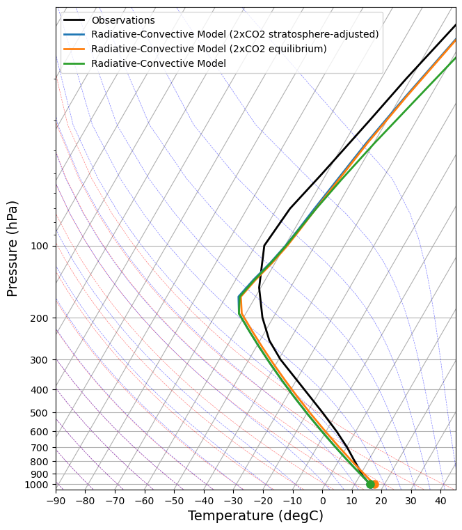
skew = make_skewT()
add_profile(skew, rcm_2xCO2_strat)
add_profile(skew, rcm_2xCO2_eq)
add_profile(skew, rcm)
ECS_nofeedback = rcm_2xCO2_eq.Ts - rcm.Ts
print('ECS with no feedback')
print(ECS_nofeedback)
print('rcm_2xCO2_eq.OLR - rcm.OLR')
print(rcm_2xCO2_eq.OLR - rcm.OLR)
print('rcm_2xCO2_eq.ASR - rcm.ASR')
print(rcm_2xCO2_eq.ASR - rcm.ASR)
lambda0 = DeltaR / ECS_nofeedback
print('lambda0')
print(lambda0)
Integrating for 1826 steps, 1826.2110000000002 days, or 5 years.
Total elapsed time is 12.736753858124827 years.
rcm_2xCO2_eq.ASR - rcm_2xCO2_eq.OLR
[1.31308298e-11]
ECS with no feedback
[1.29984831]
rcm_2xCO2_eq.OLR - rcm.OLR
[0.05080282]
rcm_2xCO2_eq.ASR - rcm.ASR
[0.05080282]
lambda0
[3.29913401]
Climate feedback#
I guess that the feedback concept is inherited from electronic engineering. For example, Professor Gu-Yeon Wei’s lecture 18 introduced the feedback concept (here):
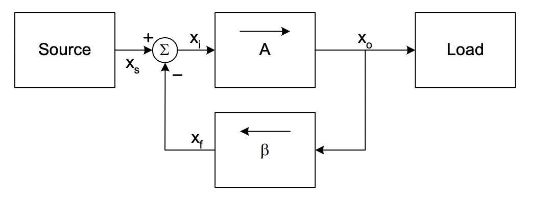
In climate science, we can think of “Source” as forcing or input added to the system, A as the whole process in the system, \(\beta\) (gain) as the amplifier or deamplifier, and the load is the output.
We use \(f\) to quantify the effect and strength of \(\beta\) (gain). If it is positive (\(f>0\)), we call it amplifying feedback. If it is negative (\(f<0\)), we call it dampling feedback.
Can you give examples for positive and negative feedbacks in the atmosphere or climate system?
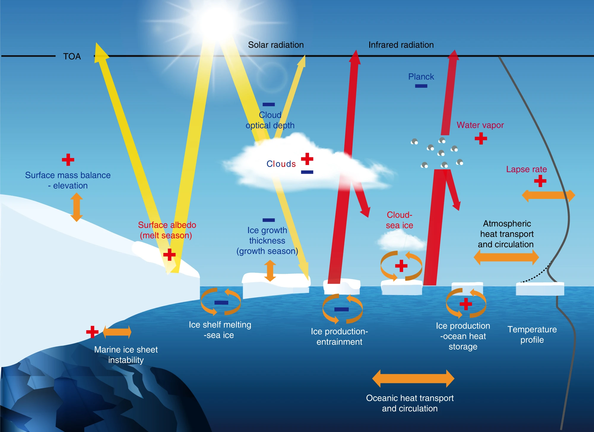
In Arctic climate system, the feedbacks could be complex. In Goosse et al. (2018), they summarized some feedbacks in the Arctic:
Let’s work on how to quantify the effect of feedbacks. We strat with the temperature change considered in a system without feedback:
We assume that a positive feedback (e.g., water vapor feedback) is included and taking action. So its effect is to “enhance” the temperature change positively with a fraction of \(f\):
Note
With infinity loops, we take the sume of each feedback effect:
Sum the original response to forcing \(\Delta R = \lambda_{0}\Delta T_{0}\),
So the final response is
We define the gain as:
What does this mean? How about a negative feedback?
If the system has N individual feedbacks, the total effect can be summed:
The ECS now becomes:
We can define feedback parameter in the unit of W/m\(^2\)/K as:
Then:
So the total feedback (parameter) could be decompose into:
Note
\(\lambda_{0}=3.3\) W/m\(^2\)/K is the Planck feedback parameter. This is not a real feedback (right?), and simply as a consequence of a warmer world emits more longwave radiation than a colder world.
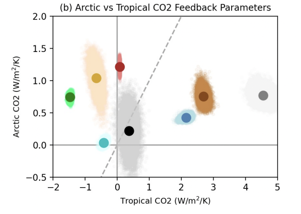
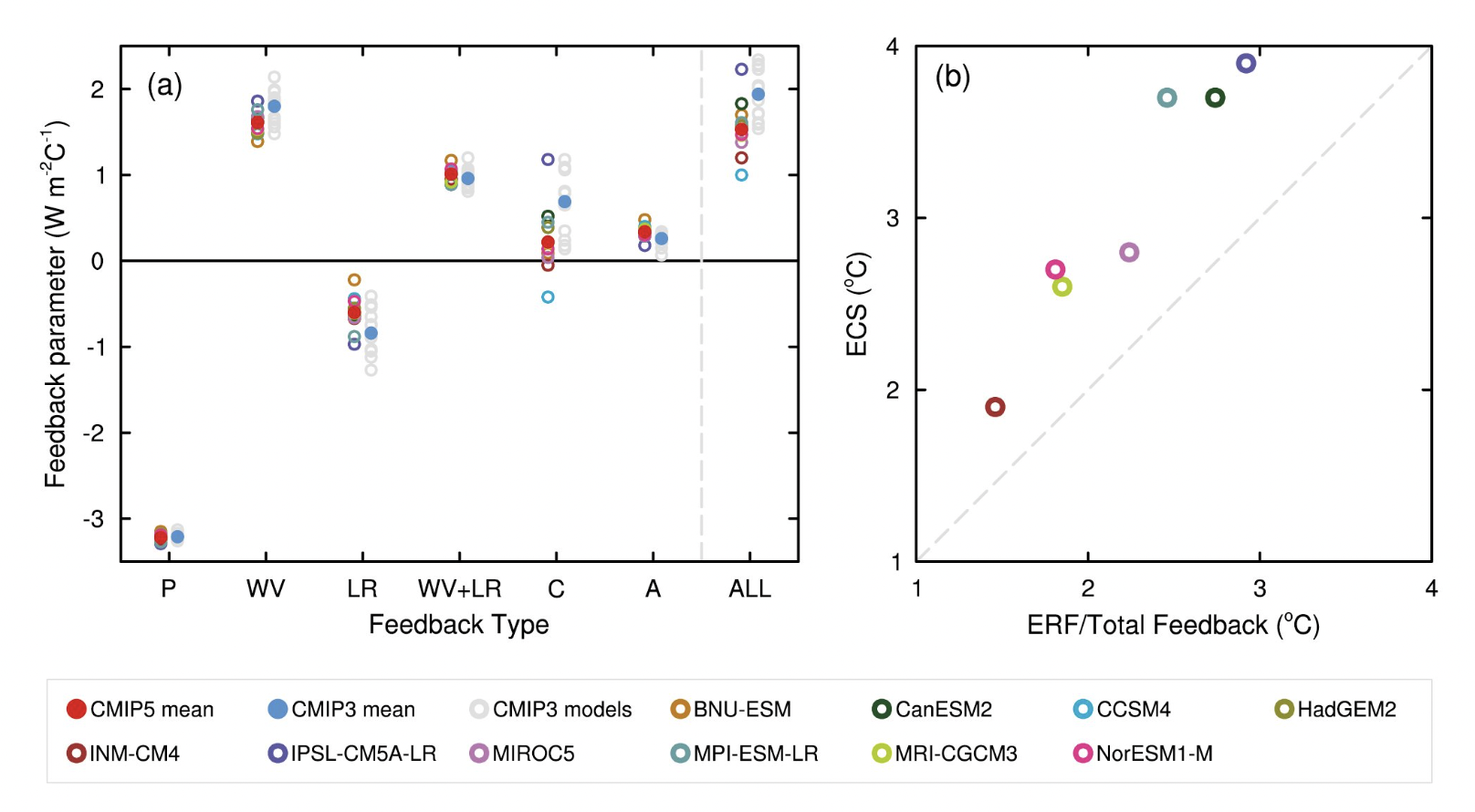
This formulation is very useful, becasue we can qunatitatively compare the importance of each feedback. Below is an example from my paper:
Now let’s add a water vapor feedback into our RCE model and calculate ECS and feedback parameter.
#  actual specific humidity
q = rcm.subprocess['Radiation'].specific_humidity
#  saturation specific humidity (a function of temperature and pressure)
qsat = climlab.utils.thermo.qsat(rcm.Tatm, rcm.lev)
#  Relative humidity
rh = q/qsat

#  Plot relative humidity in percent
fig,ax = plt.subplots()
ax.plot(q*1000, rcm.lev, 'b-')
ax.invert_yaxis()
ax.grid()
ax.set_ylabel('Pressure (hPa)')
ax.set_xlabel('Specific humidity (g/kg)', color='b')
ax.tick_params('x', colors='b')
ax2 = ax.twiny()
ax2.plot(rh*100., rcm.lev, 'r-')
ax2.set_xlabel('Relative humidity (%)', color='r')
ax2.tick_params('x', colors='r')
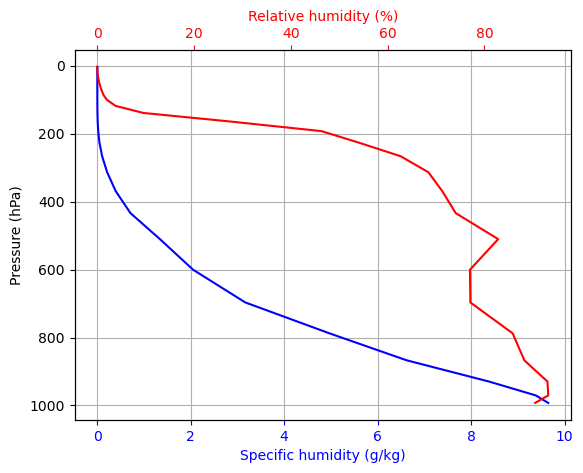
We consider the relative humidity somewhat fixed, while saturation specific humidity varied with temperature changes.
rcm_2xCO2_h2o = climlab.process_like(rcm_2xCO2)
rcm_2xCO2_h2o.name = 'RCE Model (2xCO2 equilibrium with H2O feedback)'
for n in range(2000):
# At every timestep
# we calculate the new saturation specific humidity for the new temperature
# and change the water vapor in the radiation model
# so that relative humidity is always the same
qsat = climlab.utils.thermo.qsat(rcm_2xCO2_h2o.Tatm, rcm_2xCO2_h2o.lev)
rcm_2xCO2_h2o.subprocess['Radiation'].specific_humidity[:] = rh * qsat
rcm_2xCO2_h2o.step_forward()
# Check for energy balance
print(rcm_2xCO2_h2o.ASR - rcm_2xCO2_h2o.OLR)
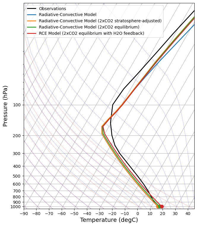
skew = make_skewT()
add_profile(skew, rcm)
add_profile(skew, rcm_2xCO2_strat)
add_profile(skew, rcm_2xCO2_eq)
add_profile(skew, rcm_2xCO2_h2o)
[-1.73180638e-07]
ECS = rcm_2xCO2_h2o.Ts - rcm.Ts
print('ECS')
print(ECS)

g = ECS / ECS_nofeedback
print('gain')
print(g)

lambda_net = DeltaR / ECS
print('lambda_net')
print(lambda_net)

print('lambda0')
print(lambda0)

lambda_h2o = lambda0 - lambda_net
print('lambda_h2o')
print(lambda_h2o)
ECS
[2.98902357]
gain
[2.29951722]
lambda_net
[1.43470724]
lambda0
[3.29913401]
lambda_h2o
[1.86442677]
“For every 1 degree of surface warming, the increased water vapor greenhouse effect provides an additional 1.86 W m\(^{-2}\) of radiative forcing.”
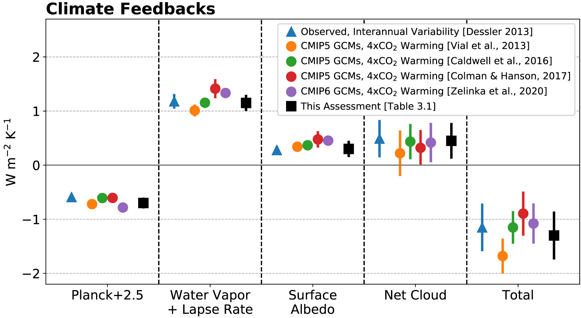
Flato et al. (2013) in IPCC AR5 reported the climate feedbacks:
Sherwood et al. (2020) summarize the climate feedbacks:
The physical model - putting together#
We review Section 2.2 of Sherwood et al. (2020) to put everything together. This is the conventional model for feedback-forcing theory.
where \(\Delta N\) is the net downward radiation imbalance at TOA, \(\Delta F\) is the radiative forcing, and \(\Delta R\) is the radiative response due to direct or indirect changes in temperature, and \(V\) is the unrelated processes.
Assume that the radiative response \(\Delta R\) is proportional to first order of the forced change in global mean surface air temperature (\(\Delta T_s\), using Taylor expansion), we can get:
Note
What is the sign of \(\lambda\)? Can the system reach to an equilibrium state if \(\lambda\) is positive?
Consider the climate system reaches an equilibrium state over a sufficient long time, so we can neglect \(\Delta N\) and \(V\).
So the climate sensitivity of doubling CO2 can be expressed as below:
The feedback \(\lambda\) can be decomposed into each feedback process:
Feebacks can change strength in different climate state –> state dependence \(\Delta \lambda_{state}\)
\(\Delta N\) can not only depend on global-mean surface air temperature but also the geographic distribution or pattern –> pattern effect \(\Delta \lambda_{pattern}\)
We can modify the model as:
where
How to calculate \(\Delta \lambda_{state}\) and \(\Delta \lambda_{pattern}\) is another long story.
Radiative kernel analysis#
Homework assignment X (due xxx)#
Please change adj_lapse_rate = 9.8. This is the dry adiabatic lapse rate. Calculate the water feedback parameter in this scenario.