17. Diffusive Response

Contents

17. Diffusive Response#

Note

The Python scripts used below and some materials are modified from Prof. Brian E. J. Rose’s climlab website.

%matplotlib inline
import numpy as np
import matplotlib.pyplot as plt
import climlab

#  for convenience, set up a dictionary with our reference parameters
param = {'A':210, 'B':2, 'a0':0.3, 'a2':0.078, 'ai':0.62, 'Tf':-10.}
model1 = climlab.EBM_annual(name='Annual EBM with ice line', 
                            num_lat=180, D=0.55, **param )
print( model1)

print(model1.param)

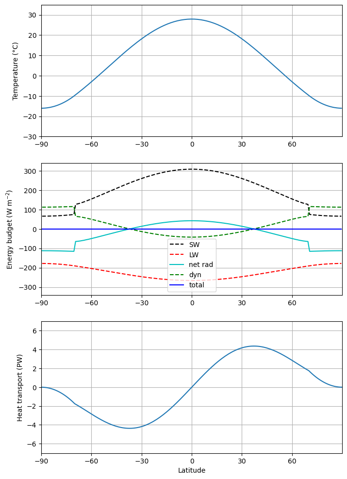
def ebm_plot( model, figsize=(8,12), show=True ):
    '''This function makes a plot of the current state of the model,
    including temperature, energy budget, and heat transport.'''
    templimits = -30,35
    radlimits = -340, 340
    htlimits = -7,7
    latlimits = -90,90
    lat_ticks = np.arange(-90,90,30)
    
    fig = plt.figure(figsize=figsize)
    
    ax1 = fig.add_subplot(3,1,1)
    ax1.plot(model.lat, model.Ts)
    ax1.set_xlim(latlimits)
    ax1.set_ylim(templimits)
    ax1.set_ylabel('Temperature (°C)')
    ax1.set_xticks( lat_ticks )
    ax1.grid()
    
    ax2 = fig.add_subplot(3,1,2)
    ax2.plot(model.lat, model.ASR, 'k--', label='SW' )
    ax2.plot(model.lat, -model.OLR, 'r--', label='LW' )
    ax2.plot(model.lat, model.net_radiation, 'c-', label='net rad' )
    ax2.plot(model.lat, model.heat_transport_convergence, 'g--', label='dyn' )
    ax2.plot(model.lat, model.net_radiation
                        + model.heat_transport_convergence, 'b-', label='total' )
    ax2.set_xlim(latlimits)
    ax2.set_ylim(radlimits)
    ax2.set_ylabel('Energy budget (W m$^{-2}$)')
    ax2.set_xticks( lat_ticks )
    ax2.grid()
    ax2.legend()
    
    ax3 = fig.add_subplot(3,1,3)
    ax3.plot(model.lat_bounds, model.heat_transport)
    ax3.set_xlim(latlimits)
    ax3.set_ylim(htlimits)
    ax3.set_ylabel('Heat transport (PW)')
    ax3.set_xlabel('Latitude')
    ax3.set_xticks( lat_ticks )
    ax3.grid()

    return fig

model1.integrate_years(5)
f = ebm_plot(model1)

model1.icelat

climlab Process of type <class 'climlab.model.ebm.EBM_annual'>. 
State variables and domain shapes: 
  Ts: (180, 1) 
The subprocess tree: 
Annual EBM with ice line: <class 'climlab.model.ebm.EBM_annual'>
   LW: <class 'climlab.radiation.aplusbt.AplusBT'>
   insolation: <class 'climlab.radiation.insolation.AnnualMeanInsolation'>
   albedo: <class 'climlab.surface.albedo.StepFunctionAlbedo'>
      iceline: <class 'climlab.surface.albedo.Iceline'>
      warm_albedo: <class 'climlab.surface.albedo.P2Albedo'>
      cold_albedo: <class 'climlab.surface.albedo.ConstantAlbedo'>
   SW: <class 'climlab.radiation.absorbed_shorwave.SimpleAbsorbedShortwave'>
   diffusion: <class 'climlab.dynamics.meridional_heat_diffusion.MeridionalHeatDiffusion'>

{'timestep': 350632.51200000005, 'S0': 1365.2, 's2': -0.48, 'A': 210, 'B': 2, 'D': 0.55, 'Tf': -10.0, 'water_depth': 10.0, 'a0': 0.3, 'a2': 0.078, 'ai': 0.62}
Integrating for 450 steps, 1826.2110000000002 days, or 5 years.

Total elapsed time is 5.000000000000044 years.

array([-70.,  70.])

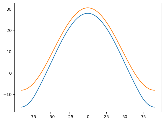
../_images/be35e15513c9b562c0e666591a7266828897fea24ec48fec7beca0a194ee0cb2.png

deltaA = 4.

model2 = climlab.process_like(model1)
model2.subprocess['LW'].A = param['A'] - deltaA
model2.integrate_years(5, verbose=False)

plt.plot(model1.lat, model1.Ts)
plt.plot(model2.lat, model2.Ts)

model2.icelat

array([-90.,  90.])

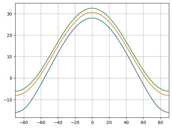
../_images/3ae39f8a96857b1fdacb5d2f25b0c6d693ab9e21a22f9cc1c463cb5edbb113d1.png

model3 = climlab.process_like(model1)
model3.subprocess['LW'].A = param['A'] - 2*deltaA
model3.integrate_years(5, verbose=False)

plt.plot(model1.lat, model1.Ts)
plt.plot(model2.lat, model2.Ts)
plt.plot(model3.lat, model3.Ts)
plt.xlim(-90, 90)
plt.grid()

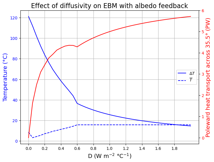
../_images/37755b5e09f59ae7ed7aa0692b8959ab1bd2533568be07078dc7d56b9c79755b.png

The effect of diffusivity with albedo feedback#

We repeat the results of Stone (1978)

param = {'A':210, 'B':2, 'a0':0.3, 'a2':0.078, 'ai':0.62, 'Tf':-10.}
print( param)

Darray = np.arange(0., 2.05, 0.05)

model_list = []
Tmean_list = []
deltaT_list = []
Hmax_list = []

for D in Darray:
    ebm = climlab.EBM_annual(num_lat=180, D=D, **param )
    ebm.integrate_years(5., verbose=False)
    Tmean = ebm.global_mean_temperature()
    deltaT = np.max(ebm.Ts) - np.min(ebm.Ts)
    HT = np.squeeze(ebm.heat_transport)
    ind = np.where(ebm.lat_bounds==35.)[0]
    Hmax = HT[ind]
    model_list.append(ebm)
    Tmean_list.append(Tmean)
    deltaT_list.append(deltaT)
    Hmax_list.append(Hmax)

color1 = 'b'
color2 = 'r'

fig = plt.figure(figsize=(8,6))
ax1 = fig.add_subplot(111)
ax1.plot(Darray, deltaT_list, color=color1, label=r'$\Delta T$')
ax1.plot(Darray, Tmean_list, '--', color=color1, label=r'$\overline{T}$')
ax1.set_xlabel('D (W m$^{-2}$ °C$^{-1}$)', fontsize=14)
ax1.set_xticks(np.arange(Darray[0], Darray[-1], 0.2))
ax1.set_ylabel(r'Temperature (°C)', fontsize=14,  color=color1)
for tl in ax1.get_yticklabels():
    tl.set_color(color1)
ax1.legend(loc='center right')
ax2 = ax1.twinx()
ax2.plot(Darray, Hmax_list, color=color2)
ax2.set_ylabel('Poleward heat transport across 35.5° (PW)', fontsize=14, color=color2)
for tl in ax2.get_yticklabels():
    tl.set_color(color2)
ax1.set_title('Effect of diffusivity on EBM with albedo feedback', fontsize=16)
ax1.grid()

{'A': 210, 'B': 2, 'a0': 0.3, 'a2': 0.078, 'ai': 0.62, 'Tf': -10.0}

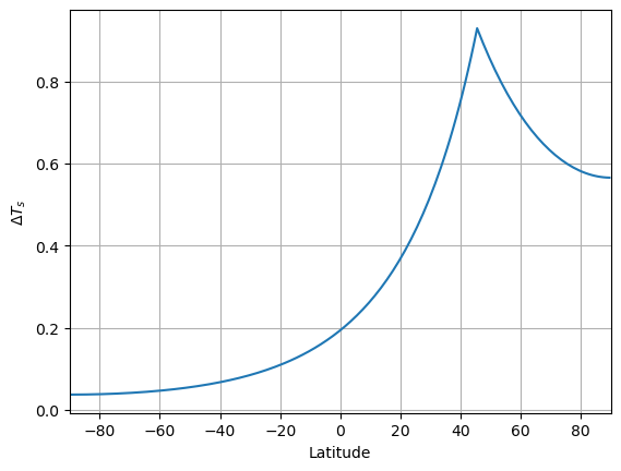
../_images/b23a48e324b0e4e0df4d736f1de4f27fa54171c5b1ec991bbbce47d59f4847a7.png

Diffusive response to a point source of energy at 45\(^o\)N#

without albedo feedback

param_noalb = {'A': 210, 'B': 2, 'D': 0.55, 'Tf': -10.0, 'a0': 0.3, 'a2': 0.078}
m1 = climlab.EBM_annual(num_lat=180, **param_noalb)
print(m1)

m1.integrate_years(5.)

m2 = climlab.process_like(m1)

point_source = climlab.process.energy_budget.ExternalEnergySource(state=m2.state, timestep=m2.timestep)
ind = np.where(m2.lat == 45.5)
point_source.heating_rate['Ts'][ind] = 100.

m2.add_subprocess('point source', point_source)
print( m2)

m2.integrate_years(5.)

plt.plot(m2.lat, m2.Ts - m1.Ts)
plt.xlim(-90,90)
plt.xlabel('Latitude')
plt.ylabel(r'$\Delta T_s$')
plt.grid()

climlab Process of type <class 'climlab.model.ebm.EBM_annual'>. 
State variables and domain shapes: 
  Ts: (180, 1) 
The subprocess tree: 
Untitled: <class 'climlab.model.ebm.EBM_annual'>
   LW: <class 'climlab.radiation.aplusbt.AplusBT'>
   insolation: <class 'climlab.radiation.insolation.AnnualMeanInsolation'>
   albedo: <class 'climlab.surface.albedo.P2Albedo'>
   SW: <class 'climlab.radiation.absorbed_shorwave.SimpleAbsorbedShortwave'>
   diffusion: <class 'climlab.dynamics.meridional_heat_diffusion.MeridionalHeatDiffusion'>

Integrating for 450 steps, 1826.2110000000002 days, or 5.0 years.

Total elapsed time is 5.000000000000044 years.
climlab Process of type <class 'climlab.model.ebm.EBM_annual'>. 
State variables and domain shapes: 
  Ts: (180, 1) 
The subprocess tree: 
Untitled: <class 'climlab.model.ebm.EBM_annual'>
   LW: <class 'climlab.radiation.aplusbt.AplusBT'>
   insolation: <class 'climlab.radiation.insolation.AnnualMeanInsolation'>
   albedo: <class 'climlab.surface.albedo.P2Albedo'>
   SW: <class 'climlab.radiation.absorbed_shorwave.SimpleAbsorbedShortwave'>
   diffusion: <class 'climlab.dynamics.meridional_heat_diffusion.MeridionalHeatDiffusion'>
   point source: <class 'climlab.process.energy_budget.ExternalEnergySource'>

Integrating for 450 steps, 1826.2110000000002 days, or 5.0 years.

Total elapsed time is 9.999999999999863 years.

../_images/af108edd8262a7cea8fd9c8d88ee68318856c36faf7652376bdb25594a4d3c0c.png

Note

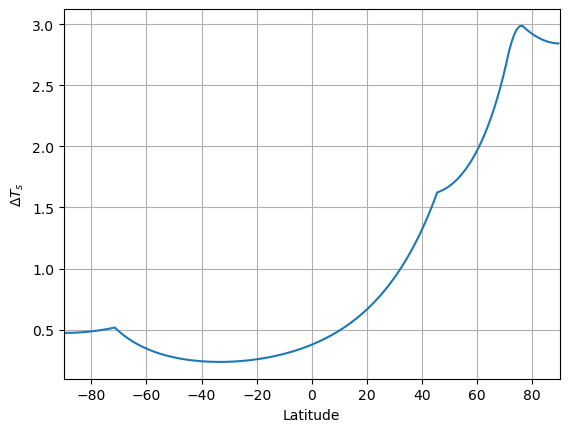
The length scale of the point warming is suggested to be proportional to \(\sqrt{\frac{D}{B}}\)

with albedo

m3 = climlab.EBM_annual(num_lat=180, **param)
m3.integrate_years(5.)
m4 = climlab.process_like(m3)
point_source = climlab.process.energy_budget.ExternalEnergySource(state=m4.state, timestep=m4.timestep)
point_source.heating_rate['Ts'][ind] = 100.
m4.add_subprocess('point source', point_source)
m4.integrate_years(5.)

plt.plot(m4.lat, m4.Ts - m3.Ts)
plt.xlim(-90,90)
plt.xlabel('Latitude')
plt.ylabel(r'$\Delta T_s$')
plt.grid()

Integrating for 450 steps, 1826.2110000000002 days, or 5.0 years.

Total elapsed time is 5.000000000000044 years.
Integrating for 450 steps, 1826.2110000000002 days, or 5.0 years.

Total elapsed time is 9.999999999999863 years.

../_images/8019daab3e13bff574abf4491a5ed65a9e8cd42f51f02fda511491a313d328e3.png