
9. Zero-dimensional Energy Balance Model#
Note
The Python scripts used below and some materials are modified from Prof. Brian E. J. Rose’s climlab website.
Global energy budget#
We start with the observed global energy budget, which is not too difficult to understand but is rather essential to many aspects of climate dynamics and modeling studies.
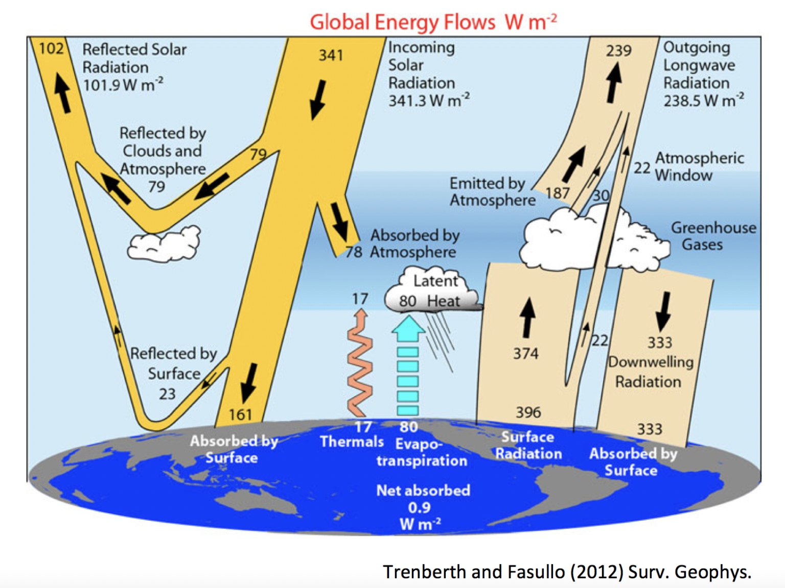
For the shortwave:
Incoming shortwave/solar radiation is 341 W/m\(^2\).
Reflected shortwave radiation is 102 W/m\(^2\).
The global mean albedo is 102 W/m\(^2\) / 341 W/m\(^2\) = 0.299 ~= 0.3.
Clouds absorption is 79 W/m\(^2\), roughly the same as atmosphere and cloud reflected 78 W/m\(^2\).
Surface receives 161 W/m\(^2\), and reflects 23 W/m\(^2\) (why smaller than cloud reflection?).
The roles of ozone (O\(_3\)) and water vapor (H\(_{2}\)O)?
For the longwave:
Surface emits 396 W/m\(^2\) (blackbody with temperture 288K?).
Emission to space is only 239 W/m\(^2\) (greenhouse effect).
Atmospheric window allos 22 W/m\(^2\) to the space directly.
Atmosphere emits downward to the surface 333 W/m\(^2\).
For others:
Evapotranspiration emits 80 W/m\(^2\) to the atmosphere (latent heat).
Thermals process emits 17 W/m\(^2\) to the atmosphere (sensible heat?).
Net radiation absorbed by the surface:
161 W/m\(^2\) (shortwave) - 17 W/m\(^2\) (sensible heat) - 80 W/m\(^2\) (latent heat) - 396 W/m\(^2\) (longwave) + 333 W/m\(^2\) (longwave from the atmosphere) = 1 W/m\(^2\) ~= W/0.9 m\(^2\)
Note
Think about the roles of clouds and water vapor.
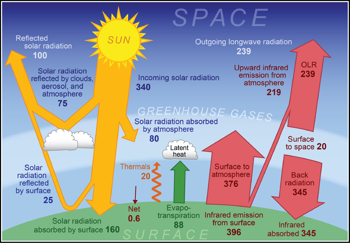
Below is the newer version of the global energy budget from Dennis L. Hartmann’s textbook:
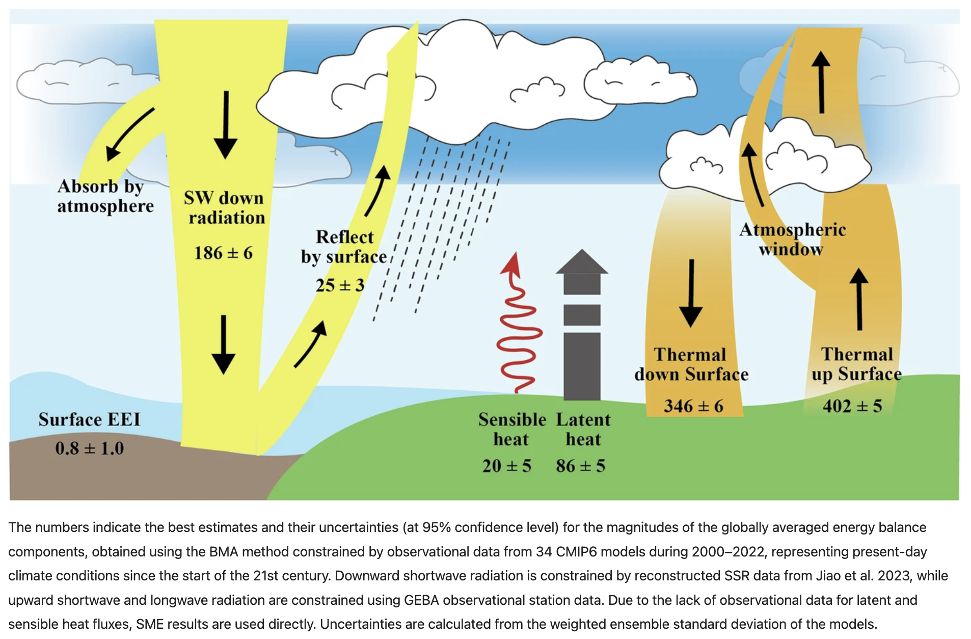
From a surface energy balance perspective, the energy budget can be estimated (from Li et al. 2024):
Calculate the energy budget#
We assume a budget for an idealised global-mean atmosphere-ocean system:
\(E\) is the heat or energy content of the system, or called enthalpy.
We will consider the energy per surface area, therefore each term has units \(\mbox{W/m}^2\).
While \(E\) is the sum of internal energy in all reservoirs (e.g., atmosphere, ocean, land, cryosphere, biosphere), the internal exchange of energy betweem them cannot be present here.
Note
Enthalpy (H) is the sum of a system’s internal energy and the product of its pressure and volume:
For the “energy flux into the system”, we assume it to be the net incoming solar radiation at the top-of-atmosphere (TOA):
\(S_{0}\) is the solar constant: 1365.2 \(\mbox{W/m}^2\).
\(A_{cross}\) is the area of illumination: \(\pi r_{p}^2\)
\(A_{surface}\) is surface area of the Earth: \(4\pi r_{p}^2\)
\(r_{p}\) is the Earth’s radius: 6371 km
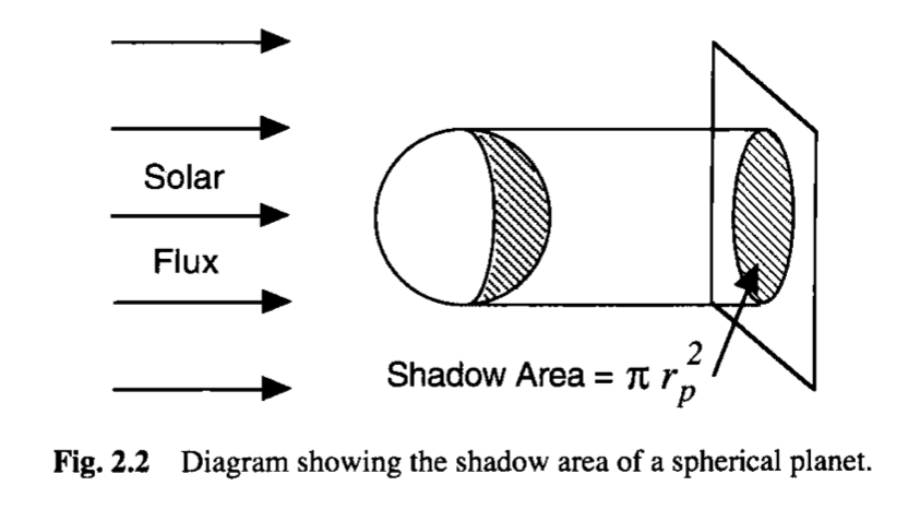
Fig. 38 Figure 2.2 from Dennis L. Hartmann’s textbook.#
For the “energy flux out of the system”, there are two components:
The amount of incoming solar radiation will be reflected back to the space \(\alpha Q\).
\(\alpha\) is the planetary albedo: reflected solar flux / incoming solar flux \(\approx 0.3\).
\(\alpha Q = 341.3*0.3 = 101.9 \mbox{W/m}^2\).
The outgoing or terrestrial longwave radiative (OLR) flux.
We assume the Earth behaves like a blackbody radiator with the emission temperature \(T_e\).
Following the Stefan-Bolzmann law: \(\sigma T_{e}^4\)
Stefan-Boltzmann constant: \(\sigma = 5.67\times 10^{-8} \mbox{W/m}^2/\mbox{K}^{4}\)
\(T_{e} = \sqrt[^4]{\frac{238.5}{\sigma}} = ?\) You should get a very cold temperature…(what happens here?)
Note
We could try to solve this puzzling by including the greenhouse effect as:
where \(\tau\) is called the transmissivity of the atmosphere.
We can use the observed value to estimate \(\tau\):
Now let’s put everything together:
We will call \((1-\alpha)Q\) the absorbed shorwave radiation (ASR).
Earth’s energy imbalance#
A recent commentary paper highlightes the energy imbalance: Mauritsen et al. (2025)
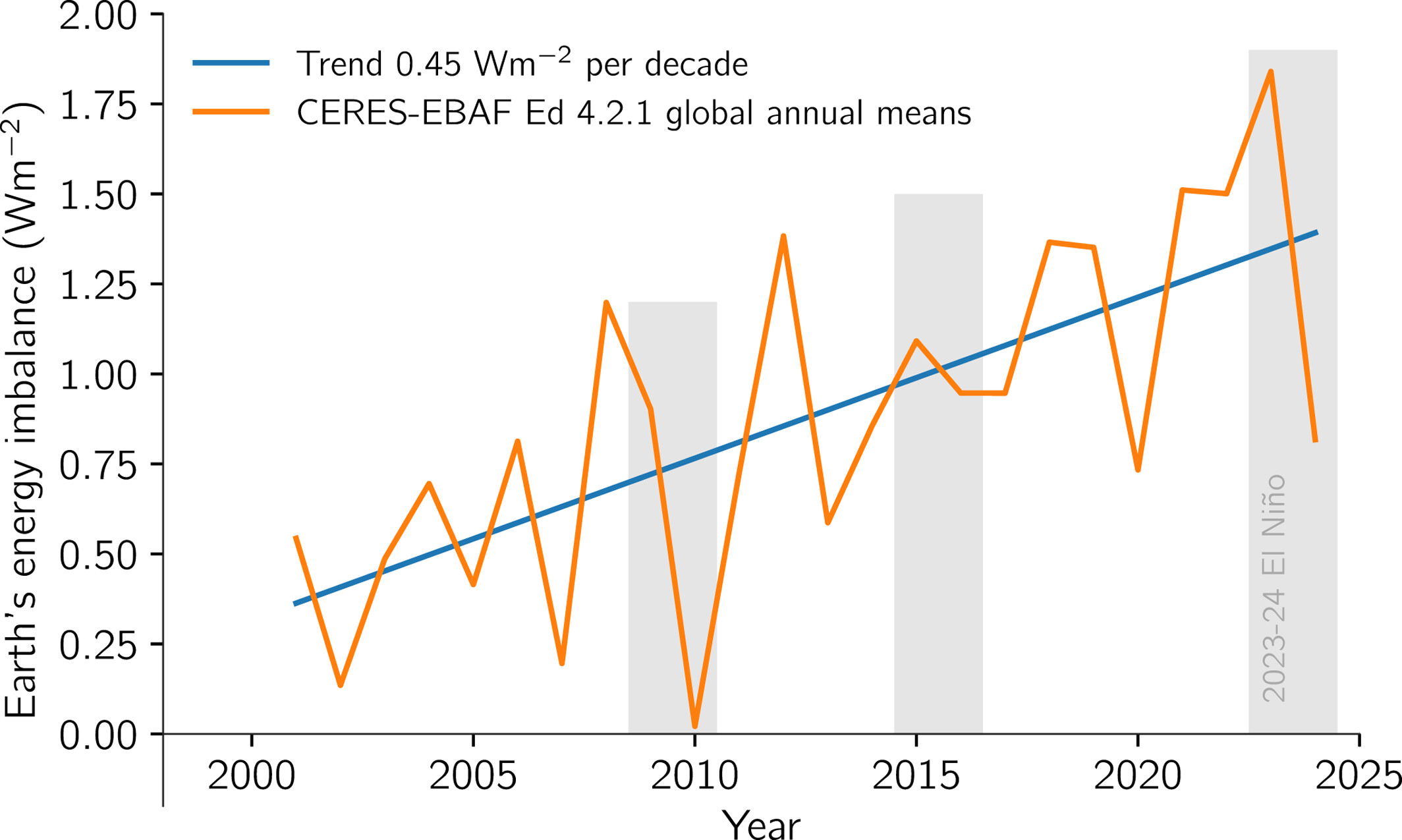
Fig. 39 Annual global mean energy imbalance observed from space during 2001–2024. The imbalance is derived from the CERES-EBAF Edition 4.2.1 data set (Loeb et al., 2018). The blue line shows the linear trend over the 2001–2024 period when full annual means are available. Gray shading shows years affected by major El Niño events. Figure from Mauritsen et al. (2025).#
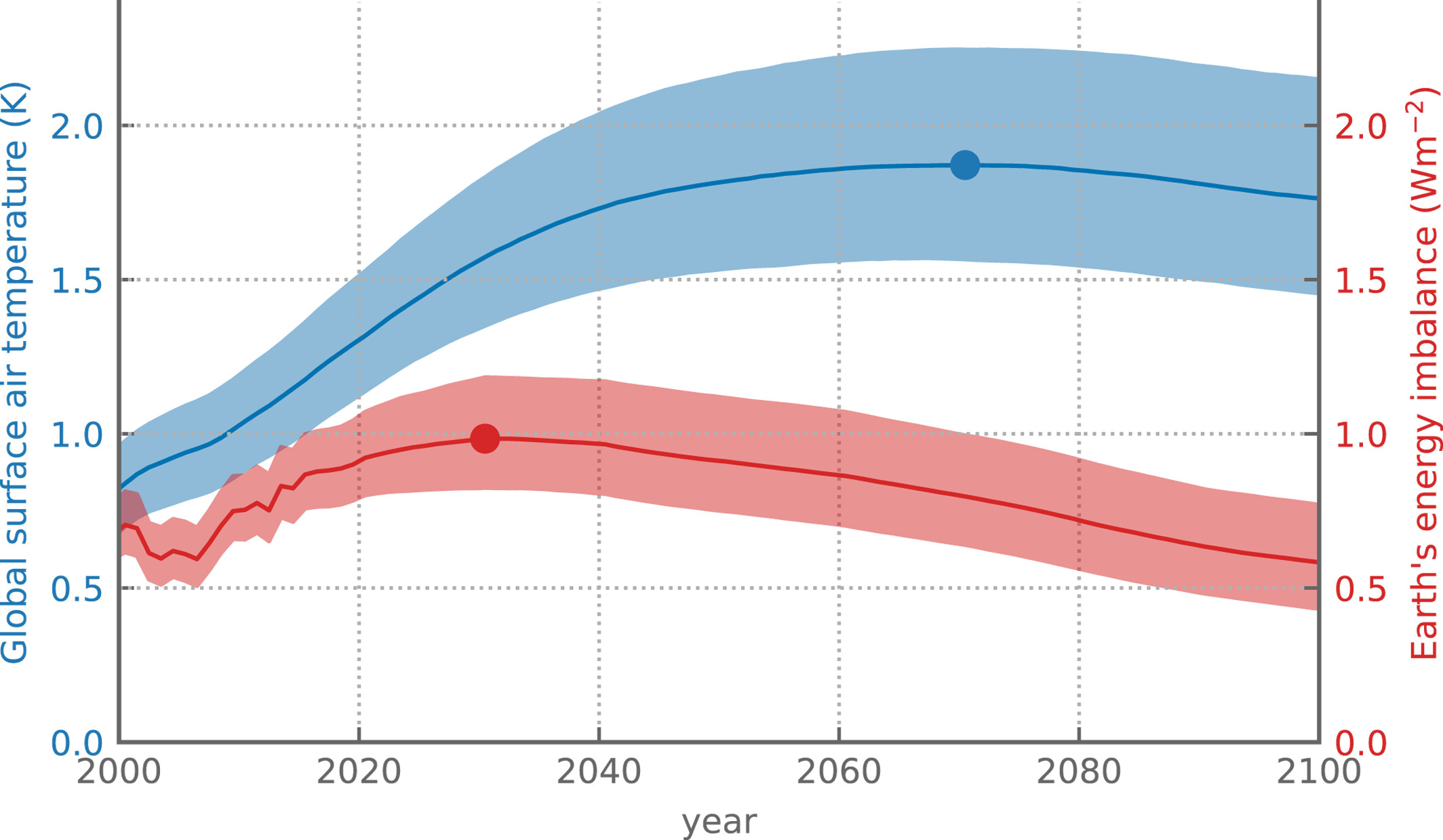
Fig. 40 Climate model global mean temperature and energy imbalance under a strong mitigation scenario meeting the 2° target (SSP1-2.6). Time series are estimated from the IPCC AR6 Earth system emulator (IPCC, 2021, Chapter 7 supplementary material). Displayed data are from (Meyssignac et al., 2023). Uncertainty ranges indicate the 90 percent confidence interval of the spread caused by uncertainties in forcing, the climate response, and the carbon cycle. The displayed uncertainty range therefore excludes internal variability. The dots mark the peak year on each time series. Figure from Mauritsen et al. (2025).#
Equilibrium state#
Assume that the Earth system is in energy balance, that is:
or
We would like to solve the surface temperature in this equilibrium state, so arrange the above equation to get:
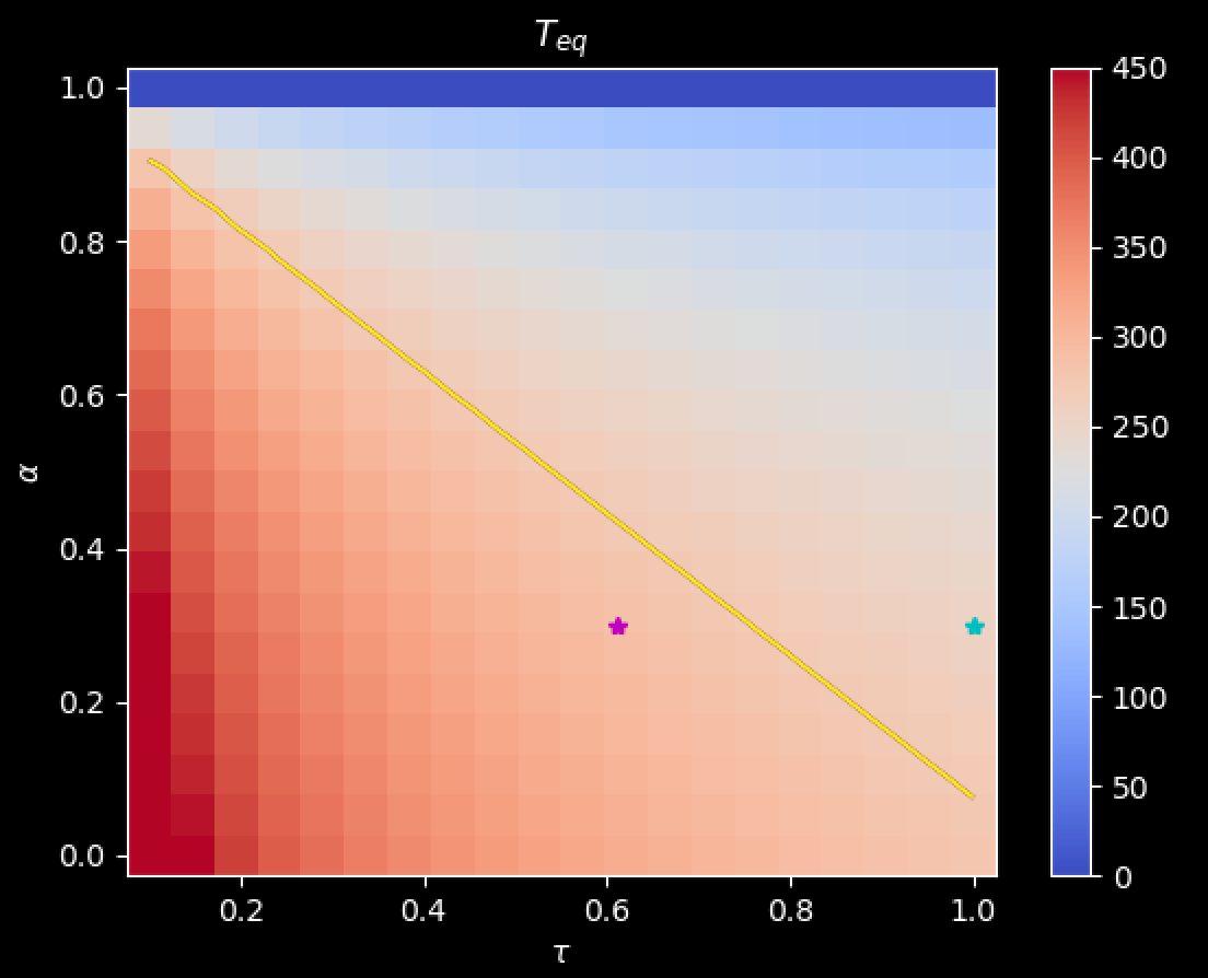
Let’s solve \(T_{eq}\) as a function of \(\alpha\) and \(\tau\).
I wrote a very bad (but easy to understand) Python code below to calcualte \(T_{eq}\) with \(\alpha\) and \(\tau\) varied (can you improve it?):
import numpy as np

nx = 20
Q = 341.3 # W / m^2
sigma = 5.67e-8 # W / m^2 / K^4
alpha = np.linspace(0,1,nx)
tau = np.linspace(0.1,1,nx)

Teq_obs = ((1-0.3)*Q/0.61/sigma)**0.25

Teq = np.zeros((nx,nx))
for JJ in range(nx):
    for II in range(nx):
        Teq[JJ,II] = ((1-alpha[JJ])*Q/tau[II]/sigma)**0.25
Can you make below figure?
Time-dependent energy balance model#
In the real word and for most climate modelling system, the energy-balance state of a climate can be broken if some disturbances or process changes in the system (e.g., greenhouse gases). The system is no longer in equilibrium, but it may adjust to a new equibrium state (if not, what will happen?). So we are now back to Equation (4).
We relate the enthalpy \(E\) to the global-mean surface temperature \(T_{s}\) with a constant \(C\):
where \(C\) is the effective heat capacity of atmosphere and ocean combined.
Note
Assuming \(C\) as a constant is somewhat tricky and highly-simplified. It is apparently not reasonable to treat the atmosphere, ocean, cryopshere together as one value \(C\). However, to start with this zero-dimensional simple model, a constant \(C\) may be suffient.
We can assume that most of the heat capacity comes from the upper ocean (reasonable, right?), then
where
\(c_w\) is the specific heat of water = \(4\times 10^{3}\) \(\mbox{J/kg/K}\).
\(\rho\) is the density of water = \(10^3\) \(\mbox{kg/m}^3\).
\(H\) is the effective depth of sea water \(\approx\) 100 m.
We will have the effective heat capacity \(4.0\times 10^{8}\) \(\mbox{J/m}^{2}\mbox{/K}\).
Then Equation (4) becomes:
Now we can solve this equation analytically!!! We adopt the concept of linear perturbation to the system:
Using Taylor series expansion, we can approximate
The energy balance equation can be then written as:
Recall that \(T_{eq}=\sqrt[4]{\frac{(1-\alpha)Q}{\tau \sigma}}\), such that:
We define a feedback parameter:
We next define a characteristic timescale:
The the equation becomes:
Take integral on both sides with a given initial condition \(T_{s}'(0)\):
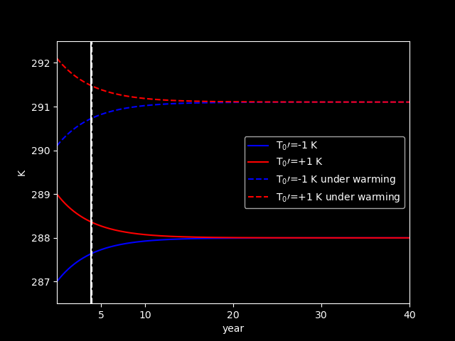
Above are all mathematics, we now discuss the parameters and outcome.
The analytical solution:
If we consider a global warming scenario, that is \(\tau=0.57\) and \(\alpha=0.32\), then we have the solutions:
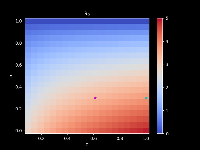
The Planck feeback, \(\lambda_{0}\):
The strength of Planck feedback can be quantified by \(\lambda_{0}\), which we usually call the Planck feedback parameter (more correctly -\(\lambda_{0}\) to denote it is a negative feedback).
If we use the code from Professor Brian Rose, we can get its value 3.31 W/m\(^2\)/K. This value does not vary too much in climate model simulations with different scenarios.
OLRobserved = 238.5  # in W/m2
sigma = 5.67E-8  # S-B constant
Tsobserved = 288.  # global average surface temperature
tau = OLRobserved / sigma / Tsobserved**4  # solve for tuned value of transmissivity

lambda_0 = 4 * sigma * tau * Tsobserved**3
#  This is an example of formatted text output in Python
print( 'lambda_0 = {:.2f} W m-2 K-1'.format(lambda_0)  )
lambda_0 = 3.31 W m-2 K-1
refer to as no-feedback climate response parameter.
Since \(\lambda_{0} = 4\tau \sigma T_{eq}^{3}\) and \(T_{eq} = \sqrt[^4]{\frac{(1-\alpha)Q}{\tau \sigma}}\), we can make a plot for \(\lambda_{0}\) as a function of \(\tau\) and \(\alpha\):
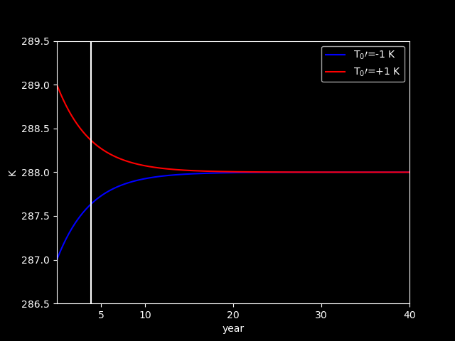
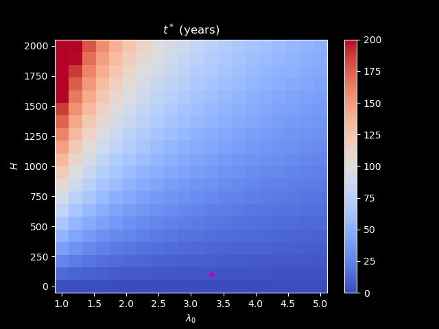
The characteristic timescale \(t^{*}\):
\(t^{*}\) depends on effective heat capacity and radiative feedback process.
We can calculate its value by \(\frac{C}{\lambda_{0}}=\frac{4.0\times10^{8}}{3.31}\approx 120845921\) second \(\approx 3.8\) year.
This means this climate system requires about 4 years to reach a quasi-equilibrium state based on the e-folding time criterion.
not too long, right?
We can make a plot to show its dependency on \(H\) and \(\lambda_{0}\):
Homework assignment 1 (due xxx)#
If the outgoing longwave radiation is 238.5 \(\mbox{W/m}^2\) as observed and we purely consider the Earth as a blackbody, what is the corresponding surface air temperature \(T_{s}\)?
Can you make the contour plot for \(T_{eq}\) as a function of \(\alpha\) and \(\tau\)? If global warming occurs, what is the possible changes in \(\alpha\) and \(\tau\), and the resultant \(T_{eq}\)?
Can you use numerical method to solve Equation (10)? Please make a plot for the numerical solution together with the analytical solution included. Please also submit your code.
Final project 1#
When global warming occurs, high temperature could melt sea ice or glaciers that greatly reduce the albedo. In other words, the planetary albedo can be considered as a function of temperature, rather than a fixed value as we discuss above.
One widely-used simple albedo parameterization is:
Discuss why we choose \(\alpha_{i}=0.7\) and \(T_{i}=260 K\). What does this condition in a climate system mean?
Discuss why we choose \(\alpha_{0} = 0.289\) and \(T_{0}=293 K\). What does this condition in a climate system mean?
Can you calcuate the solution for \(T_{eq}\) anallytically, when implementing \(\alpha(T)\) in Equation (10)?
Can you calcualte the numerical solution for \(T_{eq}\) anallytically, when implementing \(\alpha(T)\) in Equation (10)?
Please find the relationship between \(T_{eq}\) and \(\alpha(T)\).
Feel free to add or discuss anything else?