15. Seasonal cycle#
Note
The Python scripts used below and some materials are modified from Prof. Brian E. J. Rose’s climlab website.
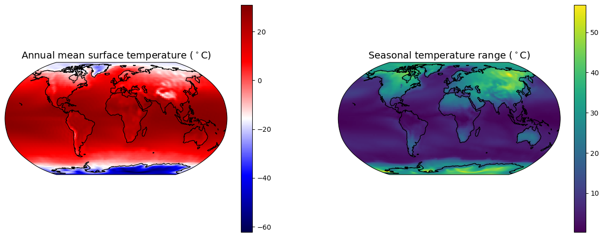
Seasonal cycle of surface air temperature from reanalysis data#
%matplotlib inline
import numpy as np
import matplotlib.pyplot as plt
import xarray as xr
import climlab
from climlab import constants as const
import cartopy.crs as ccrs # use cartopy to make some maps
ncep_url = "/Users/yuchiaol_ntuas/Desktop/ebooks/data/"
#ncep_url = "http://psl.noaa.gov/thredds/dodsC/Datasets/ncep.reanalysis.derived/"
ncep_Ts = xr.open_dataset(ncep_url + "skt.sfc.mon.1981-2010.ltm.nc", decode_times=False)
# Alternative source from the University of Hawai'i
#url = "http://apdrc.soest.hawaii.edu:80/dods/public_data/Reanalysis_Data/NCEP/NCEP/clima/"
#ncep_Ts = xr.open_dataset(url + 'surface_gauss/skt')
lat_ncep = ncep_Ts.lat; lon_ncep = ncep_Ts.lon
Ts_ncep = ncep_Ts.skt
print( Ts_ncep.shape)
maxTs = Ts_ncep.max(dim='time')
minTs = Ts_ncep.min(dim='time')
meanTs = Ts_ncep.mean(dim='time')
fig = plt.figure( figsize=(16,6) )
ax1 = fig.add_subplot(1,2,1, projection=ccrs.Robinson())
cax1 = ax1.pcolormesh(lon_ncep, lat_ncep, meanTs, cmap=plt.cm.seismic , transform=ccrs.PlateCarree())
cbar1 = plt.colorbar(cax1)
ax1.set_title('Annual mean surface temperature ($^\circ$C)', fontsize=14 )
ax2 = fig.add_subplot(1,2,2, projection=ccrs.Robinson())
cax2 = ax2.pcolormesh(lon_ncep, lat_ncep, maxTs - minTs, transform=ccrs.PlateCarree() )
cbar2 = plt.colorbar(cax2)
ax2.set_title('Seasonal temperature range ($^\circ$C)', fontsize=14)
for ax in [ax1,ax2]:
#ax.contour( lon_cesm, lat_cesm, topo.variables['LANDFRAC'][:], [0.5], colors='k');
#ax.set_xlabel('Longitude', fontsize=14 ); ax.set_ylabel('Latitude', fontsize=14 )
ax.coastlines()
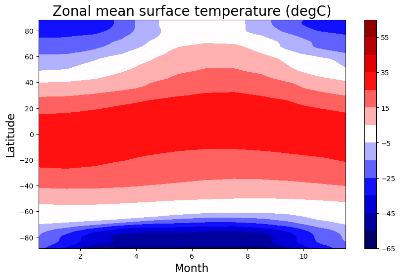
Tmax = 65; Tmin = -Tmax; delT = 10
clevels = np.arange(Tmin,Tmax+delT,delT)
fig_zonobs, ax = plt.subplots( figsize=(10,6) )
cax = ax.contourf(np.arange(12)+0.5, lat_ncep,
Ts_ncep.mean(dim='lon').transpose(), levels=clevels,
cmap=plt.cm.seismic, vmin=Tmin, vmax=Tmax)
ax.set_xlabel('Month', fontsize=16)
ax.set_ylabel('Latitude', fontsize=16 )
cbar = plt.colorbar(cax)
ax.set_title('Zonal mean surface temperature (degC)', fontsize=20)
(12, 94, 192)
Text(0.5, 1.0, 'Zonal mean surface temperature (degC)')
Analytical model#
We consider a simple model:
We have solar insolation with seasonal cycle:
where \(\omega = 2\pi\)/year, \(Q_{0}\) is the annual mean insolation.
\(\omega t = 0\) is spring equinox
\(\omega t = \pi /2\) is summer solstice
\(\omega t = \pi\) is fall equinox
\(\omega t = 3\pi/2\) is winter solstice
We seek solution in the form of:
We can determin \(T_0\) by integrating the equation for one year:
Plug the solution into the budget equation, we want to solve \(T^{*}\) and \(\Phi\):
Case \(C=0\).
In this case, the system has no heat capacity. This means that the energy cannot be stored in the system. Everything is in radiative equilibrium.
We can get
So no heat capacity gives rise to no phase shift. If we assume solar insolation amplitude is about 180 W/m\(^2\) and \(B=2\) W/m\(^2\)/K as before, we can get \(T^{*}=90\) K.
We can arrange the equation to be:
Let
This measures the efficiency of heat storage versus damping of energy anomalies through longwave radiation to space in our system.
Note
The trigonometric identities:
So we can solve the phase shift:
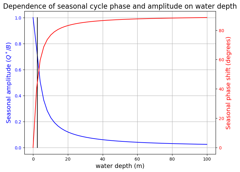
And we can solve the amplitude:
If the water depth is very very shallow:
\(\tilde{C} << 1\)
\(\Phi \approx \tilde{C}\)
\(T^{*} = \frac{Q^{*}(1-\tilde{C})}{B}\)
If the water depth is very deep:
\(\tilde{C} \to\infty\)
\(\Phi \to\ \frac{\pi}{2}\)
\(T^{*} \to 0\)
What are the physical meaning of above results?
The follow-up question is how could we get or estimate reasonalbe heat capacity?
For the atmosphere with specific heat \(c_{p} = 10^{3}\) J/kg/K,
For a well-mixed water with depth 2.5 meters:
Note
What is \(\tilde{C}\) for a lower boundary of dry land? And what is \(\tilde{C}\) for a 100-meter well-mixed ocean?
omega = 2*np.pi / const.seconds_per_year
print(omega)
B = 2.
Hw = np.linspace(0., 100.)
Ctilde = const.cw * const.rho_w * Hw * omega / B
amp = 1./((Ctilde**2+1)*np.cos(np.arctan(Ctilde)))
Phi = np.arctan(Ctilde)
color1 = 'b'
color2 = 'r'
fig = plt.figure(figsize=(8,6))
ax1 = fig.add_subplot(111)
ax1.plot(Hw, amp, color=color1)
ax1.set_xlabel('water depth (m)', fontsize=14)
ax1.set_ylabel('Seasonal amplitude ($Q^* / B$)', fontsize=14, color=color1)
for tl in ax1.get_yticklabels():
tl.set_color(color1)
ax2 = ax1.twinx()
ax2.plot(Hw, np.rad2deg(Phi), color=color2)
ax2.set_ylabel('Seasonal phase shift (degrees)', fontsize=14, color=color2)
for tl in ax2.get_yticklabels():
tl.set_color(color2)
ax1.set_title('Dependence of seasonal cycle phase and amplitude on water depth', fontsize=16)
ax1.grid()
ax1.plot([2.5, 2.5], [0, 1], 'k-');
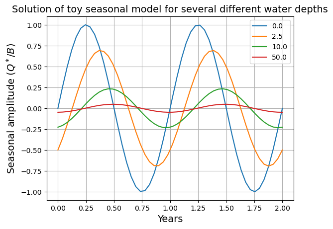
fig, ax = plt.subplots()
years = np.linspace(0,2)
Harray = np.array([0., 2.5, 10., 50.])
for Hw in Harray:
Ctilde = const.cw * const.rho_w * Hw * omega / B
Phi = np.arctan(Ctilde)
ax.plot(years, np.sin(2*np.pi*years - Phi)/np.cos(Phi)/(1+Ctilde**2), label=Hw)
ax.set_xlabel('Years', fontsize=14)
ax.set_ylabel('Seasonal amplitude ($Q^* / B$)', fontsize=14)
ax.set_title('Solution of toy seasonal model for several different water depths', fontsize=14)
ax.legend(); ax.grid()
1.991063797294792e-07
Adding heat transport back to EBM#
To make if more realistic, we assume albedo to be:
# for convenience, set up a dictionary with our reference parameters
param = {'A':210, 'B':2, 'a0':0.354, 'a2':0.25, 'D':0.6}
print(param)
# We can pass the entire dictionary as keyword arguments using the ** notation
model1 = climlab.EBM_seasonal(**param, name='Seasonal EBM')
print(model1)
# We will try three different water depths
water_depths = np.array([2., 10., 50.])
num_depths = water_depths.size
Tann = np.empty( [model1.lat.size, num_depths] )
models = []
for n in range(num_depths):
ebm = climlab.EBM_seasonal(water_depth=water_depths[n], **param)
models.append(ebm)
models[n].integrate_years(20., verbose=False )
models[n].integrate_years(1., verbose=False)
Tann[:,n] = np.squeeze(models[n].timeave['Ts'])
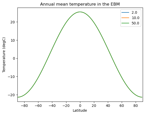
lat = model1.lat
fig, ax = plt.subplots()
ax.plot(lat, Tann)
ax.set_xlim(-90,90)
ax.set_xlabel('Latitude')
ax.set_ylabel('Temperature (degC)')
ax.set_title('Annual mean temperature in the EBM')
ax.legend( water_depths )
num_steps_per_year = int(model1.time['num_steps_per_year'])
Tyear = np.empty((lat.size, num_steps_per_year, num_depths))
for n in range(num_depths):
for m in range(num_steps_per_year):
models[n].step_forward()
Tyear[:,m,n] = np.squeeze(models[n].Ts)
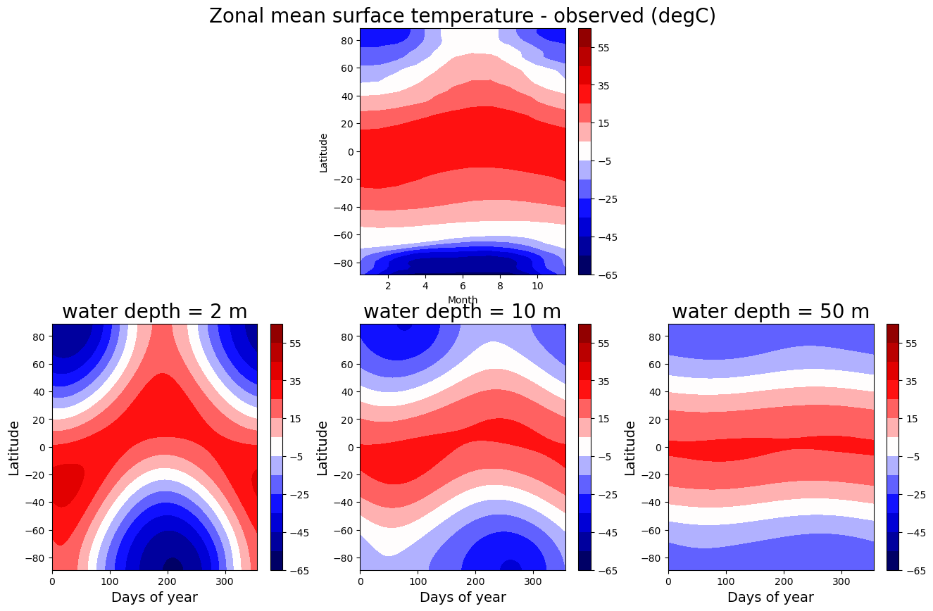
fig = plt.figure( figsize=(16,10) )
ax = fig.add_subplot(2,num_depths,2)
cax = ax.contourf(np.arange(12)+0.5, lat_ncep,
Ts_ncep.mean(dim='lon').transpose(),
levels=clevels, cmap=plt.cm.seismic,
vmin=Tmin, vmax=Tmax)
ax.set_xlabel('Month')
ax.set_ylabel('Latitude')
cbar = plt.colorbar(cax)
ax.set_title('Zonal mean surface temperature - observed (degC)', fontsize=20)
for n in range(num_depths):
ax = fig.add_subplot(2,num_depths,num_depths+n+1)
cax = ax.contourf(4*np.arange(num_steps_per_year),
lat, Tyear[:,:,n], levels=clevels,
cmap=plt.cm.seismic, vmin=Tmin, vmax=Tmax)
cbar1 = plt.colorbar(cax)
ax.set_title('water depth = %.0f m' %models[n].param['water_depth'], fontsize=20 )
ax.set_xlabel('Days of year', fontsize=14 )
ax.set_ylabel('Latitude', fontsize=14 )
{'A': 210, 'B': 2, 'a0': 0.354, 'a2': 0.25, 'D': 0.6}
climlab Process of type <class 'climlab.model.ebm.EBM_seasonal'>.
State variables and domain shapes:
  Ts: (90, 1)
The subprocess tree:
Seasonal EBM: <class 'climlab.model.ebm.EBM_seasonal'>
   LW: <class 'climlab.radiation.aplusbt.AplusBT'>
   insolation: <class 'climlab.radiation.insolation.DailyInsolation'>
   albedo: <class 'climlab.surface.albedo.P2Albedo'>
   SW: <class 'climlab.radiation.absorbed_shorwave.SimpleAbsorbedShortwave'>
   diffusion: <class 'climlab.dynamics.meridional_heat_diffusion.MeridionalHeatDiffusion'>
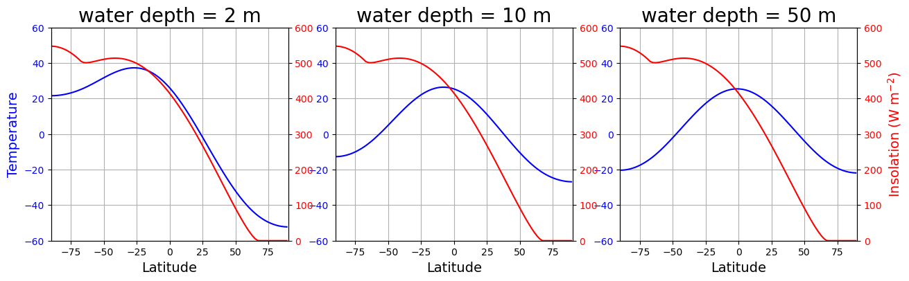
Now let’s make an animation.
def initial_figure(models):
    fig, axes = plt.subplots(1,len(models), figsize=(15,4))
    lines = []
    for n in range(len(models)):
        ax = axes[n]
        c1 = 'b'
        Tsline = ax.plot(lat, models[n].Ts, c1)[0]
        ax.set_title('water depth = %.0f m' %models[n].param['water_depth'], fontsize=20 )
        ax.set_xlabel('Latitude', fontsize=14 )
        if n == 0:
            ax.set_ylabel('Temperature', fontsize=14, color=c1 )
        ax.set_xlim([-90,90])
        ax.set_ylim([-60,60])
        for tl in ax.get_yticklabels():
            tl.set_color(c1)
        ax.grid()

        c2 = 'r'
        ax2 = ax.twinx()
        Qline = ax2.plot(lat, models[n].insolation, c2)[0]
        if n == 2:
            ax2.set_ylabel('Insolation (W m$^{-2}$)', color=c2, fontsize=14)
        for tl in ax2.get_yticklabels():
            tl.set_color(c2)
        ax2.set_xlim([-90,90])
        ax2.set_ylim([0,600])
        lines.append([Tsline, Qline])
    return fig, axes, lines

def animate(step, models, lines):
    for n, ebm in enumerate(models):
        ebm.step_forward()
        #  The rest of this is just updating the plot
        lines[n][0].set_ydata(ebm.Ts)
        lines[n][1].set_ydata(ebm.insolation)
    return lines

#  Plot initial data
fig, axes, lines = initial_figure(models)

#  Some imports needed to make and display animations
from IPython.display import HTML
from matplotlib import animation

num_steps = int(models[0].time['num_steps_per_year'])
ani = animation.FuncAnimation(fig, animate,
        frames=num_steps,
        interval=80,
        fargs=(models, lines),
        )

HTML(ani.to_html5_video())
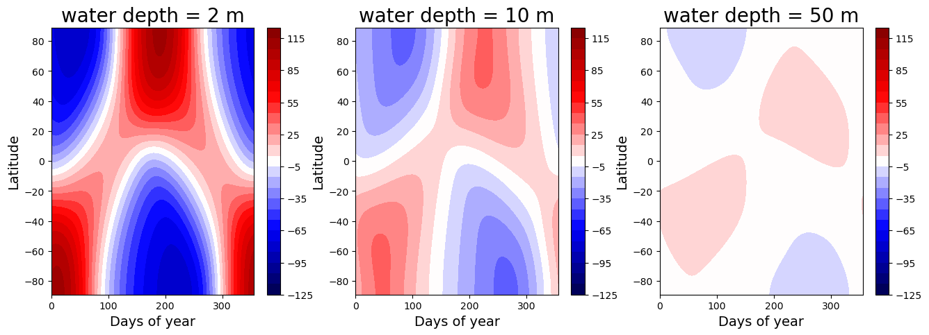
Homework assignment X (due xxx)#
Try below example and discuss the results.
orb_highobl = {'ecc':0.,
               'obliquity':90.,
               'long_peri':0.}
print( orb_highobl)
model_highobl = climlab.EBM_seasonal(orb=orb_highobl, **param)
print( model_highobl.param['orb'])

Tann_highobl = np.empty( [lat.size, num_depths] )
models_highobl = []

for n in range(num_depths):
    model = climlab.EBM_seasonal(water_depth=water_depths[n],
                                 orb=orb_highobl,
                                 **param)
    models_highobl.append(model)
    models_highobl[n].integrate_years(40., verbose=False )
    models_highobl[n].integrate_years(1., verbose=False)
    Tann_highobl[:,n] = np.squeeze(models_highobl[n].timeave['Ts'])

Tyear_highobl = np.empty([lat.size, num_steps_per_year, num_depths])
for n in range(num_depths):
    for m in range(num_steps_per_year):
        models_highobl[n].step_forward()
        Tyear_highobl[:,m,n] = np.squeeze(models_highobl[n].Ts)

fig = plt.figure( figsize=(16,5) )
Tmax_highobl = 125; Tmin_highobl = -Tmax_highobl; delT_highobl = 10
clevels_highobl = np.arange(Tmin_highobl, Tmax_highobl+delT_highobl, delT_highobl)
for n in range(num_depths):
    ax = fig.add_subplot(1,num_depths,n+1)
    cax = ax.contourf( 4*np.arange(num_steps_per_year), lat, Tyear_highobl[:,:,n],
        levels=clevels_highobl, cmap=plt.cm.seismic, vmin=Tmin_highobl, vmax=Tmax_highobl )
    cbar1 = plt.colorbar(cax)
    ax.set_title('water depth = %.0f m' %models[n].param['water_depth'], fontsize=20 )
    ax.set_xlabel('Days of year', fontsize=14 )
    ax.set_ylabel('Latitude', fontsize=14 )

lat2 = np.linspace(-90, 90, 181)
days = np.linspace(1.,50.)/50 * const.days_per_year
Q_present = climlab.solar.insolation.daily_insolation( lat2, days )
Q_highobl = climlab.solar.insolation.daily_insolation( lat2, days, orb_highobl )
Q_present_ann = np.mean( Q_present, axis=1 )
Q_highobl_ann = np.mean( Q_highobl, axis=1 )
{'ecc': 0.0, 'obliquity': 90.0, 'long_peri': 0.0}
{'ecc': 0.0, 'obliquity': 90.0, 'long_peri': 0.0}