7. Polar Stratospheric Circulation#
Note
StratObserve by Dr. Zachary D. Lawrence is very useful to monitor stratospheric conditions.
Stratospheric polar vortex#
Displacement
Splitting
2020-2021 polar vortex evolution

Sudden stratospheric warming (SSW)#
SSW and polar vortex breakdown
Days 0-30 T anomalies following SSW
“Surface Amplification” of the stratospheric signal
Definition of SSW#
The most widely used definition of SSW is following Charlton and Polvani (2007):
“the reversal of the daily-mean zonal-mean zonal winds from westerly to easterly at 60◦ N latitude and 10 hPa from November to April (by CP07, wind reversals must be separated by 20 consecutive days of westerly winds and must return to westerly for at least 10 consecutive days prior to 30 April, to be classified as a mid-winter SSW.).“
Temperature information can be dropped because of thermal wind balance!
SSW dynamical frameworks#
Large-scale planetary wave propagating upward
Planetary wave propagating upward – Charney-Drazin criterion
Baroclinic instability
Upscale cascade from synoptic-scale waves
Topography
Land-sea contrast
Planetary Wave Forcing
SSWs only happen with sufficiently strong planetary wave forcing from the troposphere.
SSWs require a pulse of anomalously strong wave forcing from the troposphere to initiate.“
Wave1 -> bottom-up
Wave2 -> top-down
Wave-mean flow interactions and dissipation
EP flux
Heat budget analysis
PV perspective
External influences on SSWs#
QBO
ENSO
11-year solar cycle
MJO
snow cover
sea ice
Dynamical downward propagation#
Tropospheric anomalies should be proportional to stratospheric ones!
Wave driving (EP flux divergence) -> downward control (x)
Wave absorption and reflection. (x)
Baroclinic eddies (v)
Stratospheric PV anomalies (v? too weak)
Surface signature of SSW’s downward influences#
Midlatitude surface impacts
Oceanic impacts
Tropical impacts
Two-way coupling of troposphere and stratosphere#
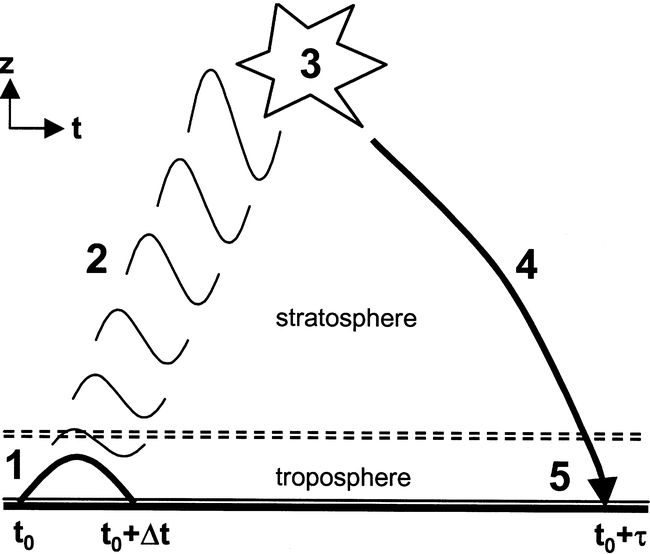
Fig. 25 Schematic illustration of the coupling events simulated in this study. (1) Forced pulse of planetary waves occurring over time Δt; (2) upward-propagating waves; (3) dissipation and breaking of waves; (4) induced downward-propagating anomalies; and (5) tropospheric response. Source: Reichler et al. (2005)#
Polar vortex and SSW in climate models#
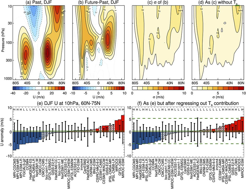
Fig. 26 This figure is from Simpson et al. (2018)#

Fig. 27 Seasonal distribution of SSWs from November to March in the MME of the historical simulation (gray bars), the RCP45/SSP245 simulation (blue bars), and the RCP85/SSP585 simulation (light blue bars) from (a) CMIP5 and (b) CMIP6. The reanalysis is shown with red bars. The differences between historical simulations and future scenarios projections are significant at the 95% confidence level for a few months, marked with a pentagram over the corresponding scenarios. Source: Rao and Garfinkel (2021).#
SSW forecast#
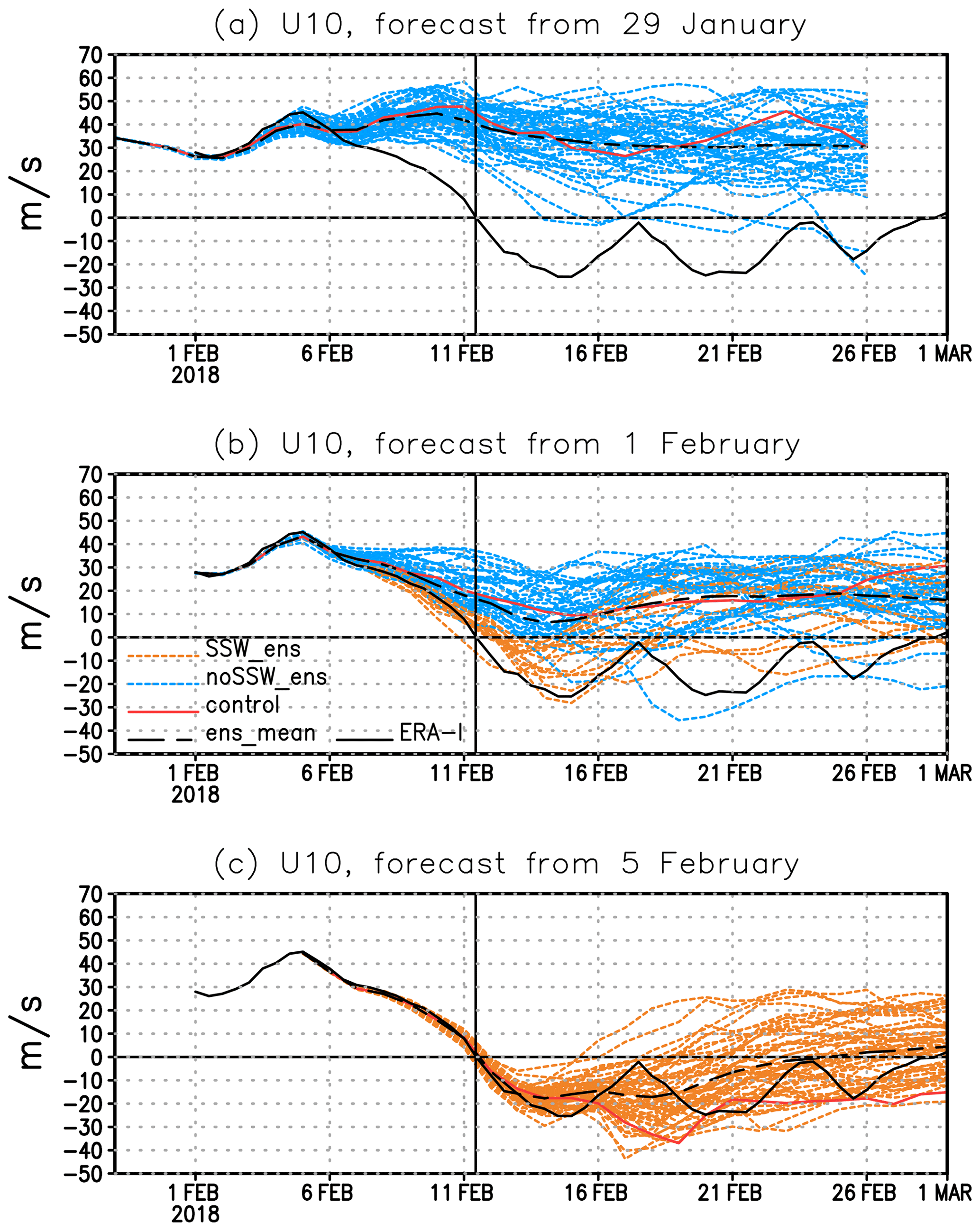
Fig. 28 Zonal-mean zonal wind at 10 hPa and 60° N (m s−1). (a) Ensemble forecast initialized on 29 January; (b) ensemble forecast initialized on 1 February (orange lines denote ensemble members that predict wind reversal with max 1 d delay, red line – control forecast, black dashed line – ensemble mean) and the ERA-I reanalysis (black solid line); (c) forecast initialized on 5 February. Vertical line denotes the SSW2018 central date. Source: Erner et al. (2020).#
SSW forecast#
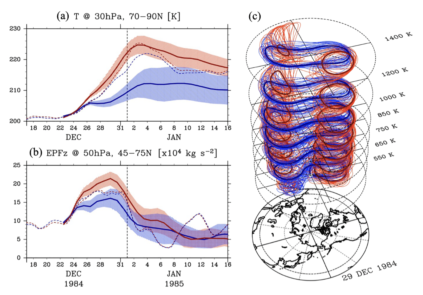
Fig. 29 Satellite impact on forecasts of SSW onset in an extreme case. JRA‐55 (red line) and JRA‐55C (blue line) ensemble forecasts starting from D−10 are shownfor an SSW that occurred on 1 January 1985. Time series of (a) 30‐hPa temperature averaged northward of 70°N and (b) vertical component of 50‐hPa E‐P fluxthat averaged over 45–75°N. Thick lines and shades indicate the ensemble mean values and 0.5 standard deviations among ensemble members. JRA‐55 andJRA‐55C are also shown by dotted lines. (c) Three‐dimensional distributions of the vortex edges (isolines of the vertically weighted potential vorticity), of thestratospheric polar vortex, for a 7‐day forecast field (validated at 3 days before D0). As a vortex edge, 38 PVU contours of Lait’s PV at isothermal surfaces are plottedfor each ensemble forecasts (cf. Matthewman et al. 2009). Thick lines indicate the ensemble means. Source: Noguchi et al. (2020).#
SSW impacts on the atmosphere above stratosphere#
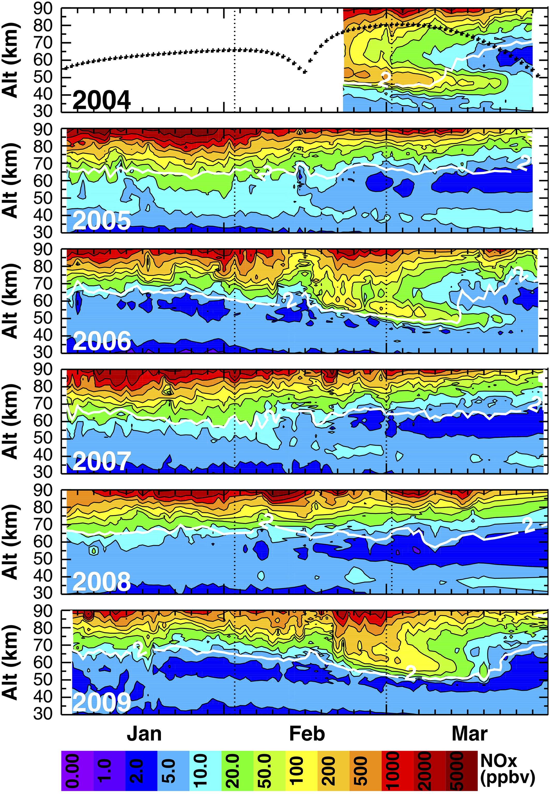
Fig. 30 Zonal average ACE-FTS NOx (color) in the NH from 1 January through 31 March of 2004–2009. The white contour indicates CO = 2.0 ppmv. Source: Baldwin et al. (2020).#