10. Layered Energy Balance Model#
The zero-dimensional energy balance model discussed in previous lecture does not contain vertical distribution of the atmosphere, which is important in understanding climate change. We will introduce the simple two-layer model, simple three-layer model, and n-layer model. These models will pave a road for understanding Manabe’s radiative-convective equilibrium that will be discussed in the next lecture. Before these, let’s start with radiation process in the atmosphere.
Atmospheric absorption spectra#
The most important results, using Planck’s law from atmospheric radiation studies are probably can be shown in the figure from Dennis L. Hartmann’s textbook (his Figure 3.1):
We call longer wavelengths “infrared”, and shorter wavelengths “ultraviolet”.
The Earth emission temperature is 255 K.
The Sun emission temperature is 6000 K with peak wavelength \(\lambda_{peak, Sun}\) 0.6 \(\mu m\).
We know that soloar spectrum peaks at 0.6 micrometers. By Wien’s displacement law, we can get:
Let’s quickly review the air gas composition looking at Hartmann’s table1.1:
The abropstion of these gases, Figure 3.4 from Hartmann’s text book:
The molecular structure of these gases, Figure 3.3 from Hartmann’s text book:
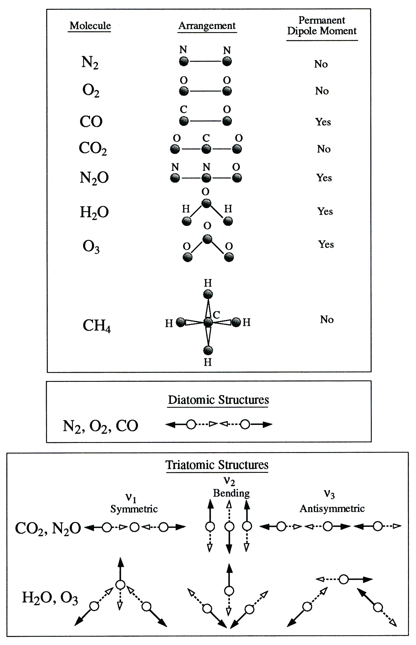
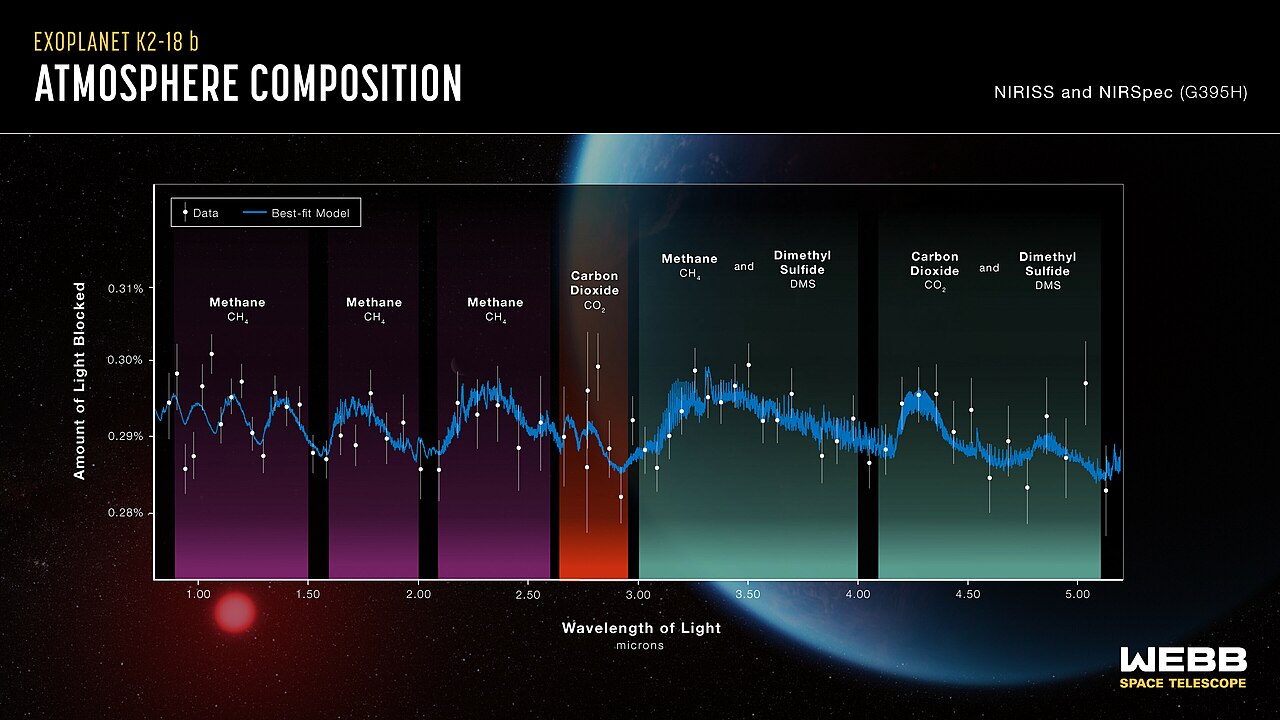
Fig. 41 K2-18b James Webb Space Telescope spectra from 2023. Credit: NASA, CSA, ESA, J. Olmstead, N. Madhusudhan 2023. Source: Wikipedia#
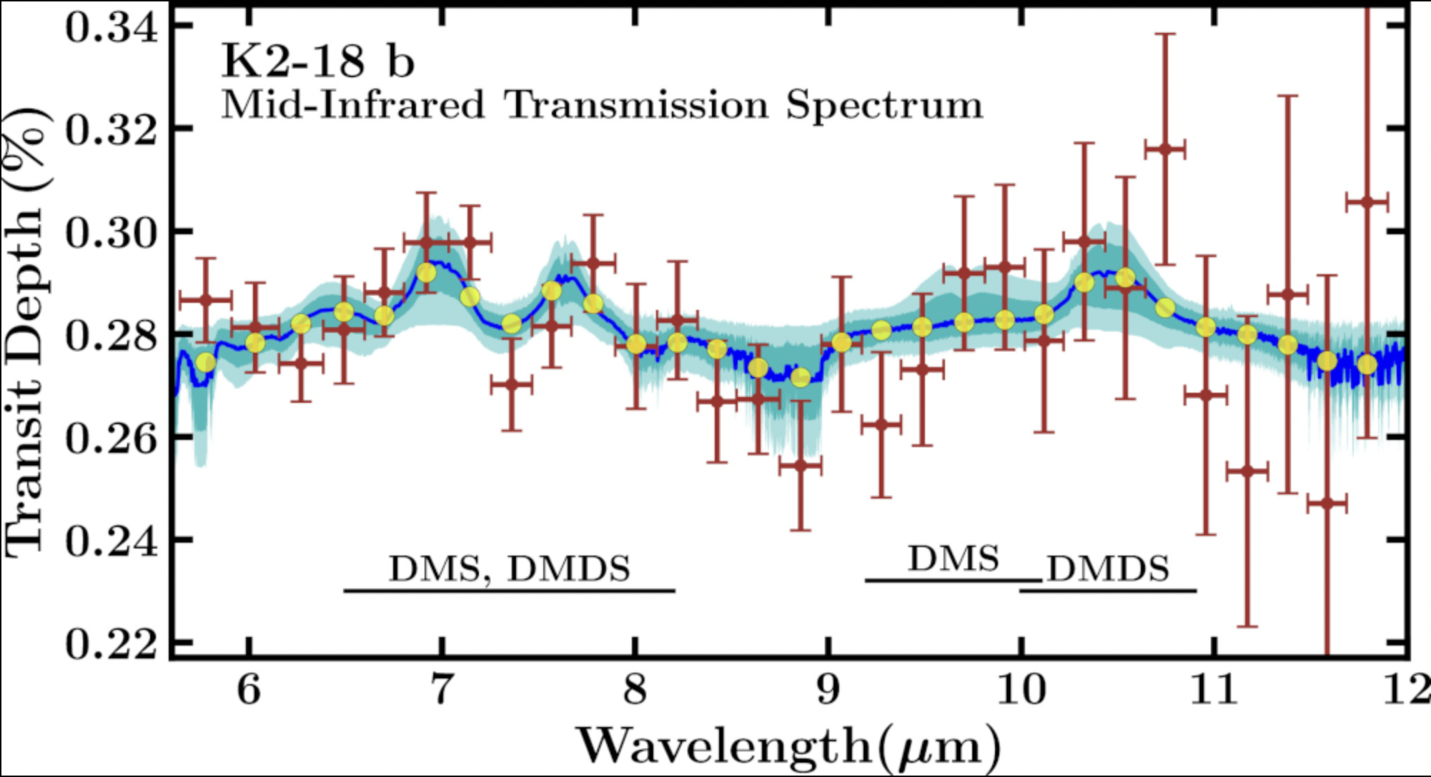
Fig. 42 The infrared transmission spectrum of the exoplanet K2-18 b taken by JWST MIRI. Credit: Madhusudhan et al. 2025. Source: Wikipedia#
Model with one-layer atmosphere and one-layer surface (one-layer model)#
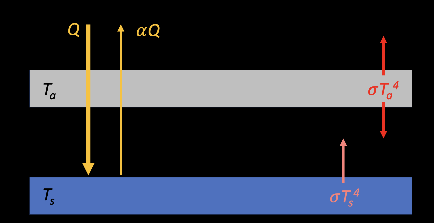
We assume:
A single-layer atmosphere with temperature \(T_{a}\).
The atmosphere is transparent to shortwave radiation.
The surface albedo is \(\alpha\).
The atmosphere absorbs all longwave radiation from the surface.
The atmosphere and surface are blackbodies.
The atmosphere radiates equally upward and downward.
We consider surface energy balance:
Note
back radiation: \(\sigma T_{a}^{4}\)
We consider atmosphere energy balance:
So we can get the result that surface temperature is alway higher than the atmospheric temperature:
If we assume \(T_{a}\) = \(T_{e}\) = 255 K (the emission temperature, how do we get this value?), we can \(T_{s}\) = 303 K. In reality, the surface temperature is about 288 K, lower than 303 K. Why?
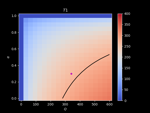
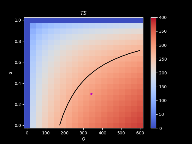
Let’s play around with varying \(Q\) and \(\alpha\):
Model with two-layer atmosphere and one-layer surface (two-layer model)#
The surface temperature is too warm in the one-layer model. How could we improve the model to better capture the real surface air temperature?
Many aspects can be considered (can you think about some?). We start by considering the vertical structure and longwave absorption by the atmosphere(s).
We keep most of the assumptions made for one-layer model, but modify the model as below:
include one more atmospheric layer.
each atmospehric layer absorbs a fraction of longwave radiation. This fraction is \(\epsilon\) and we call it absorptivity.
the reamaining \(1-\epsilon\) readiation will pass through the layer.
we adopt the Kirchhoff’s law of thermal radiation: “For an arbitrary body emitting and absorbing thermal radiation in thermodynamic equilibrium, the emissivity function is equal to the absorptivity function.”. That is absorptivity is equal to emissivity.
consider the two longwave beams: upward (U) and downward (D) beams.
Note
This is a grey gas-type model. Grey meands that the emission and absorption do not depend on the wavelength.
Let’s look at the model:
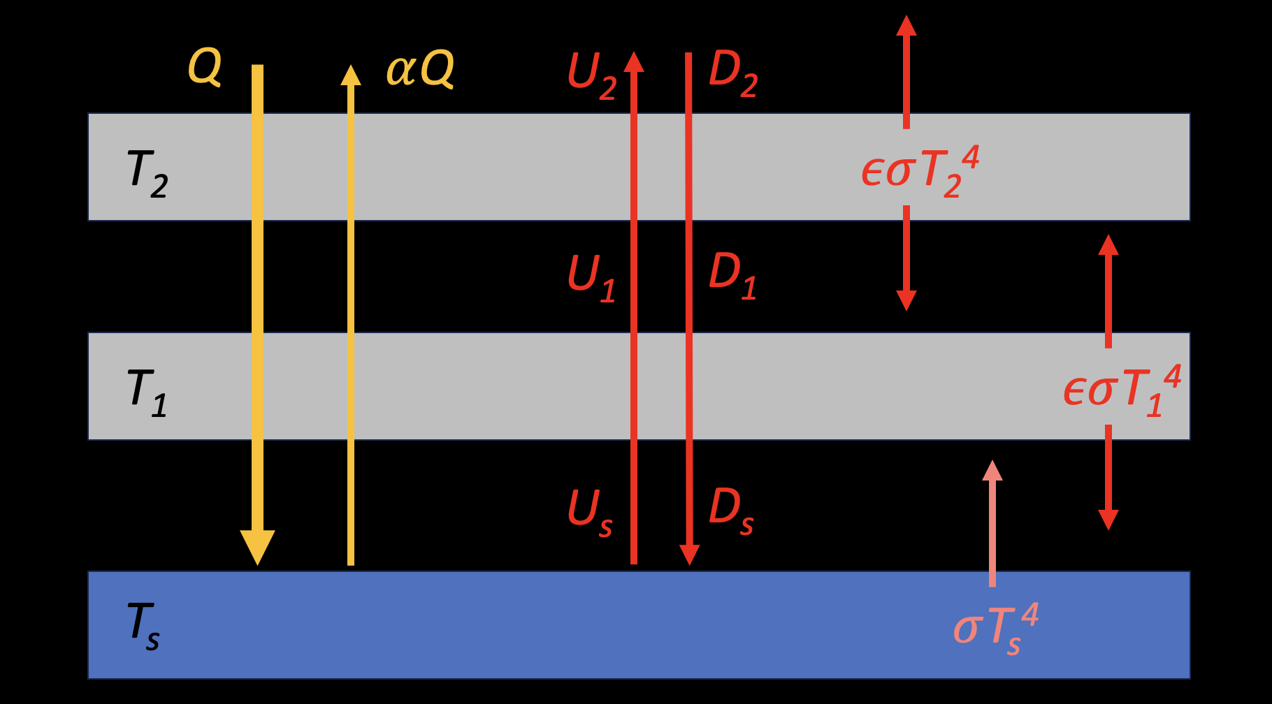
Upward beam#
Downward beam#
If \(\epsilon = 1\), the atmopsheres absorb everything:
If \(\epsilon = 0\), the atmopsheres absorb nothing:
Let’s solve temperatures considering an energy balance state!
The atmospheric layer2#
The atmospheric layer1#
The surface#
Now we can write the above equations in a matrix form:
It is a bit tedious to calculate the inverse of the matrix. We can use online tool (here) to calculate it:
So we can get:
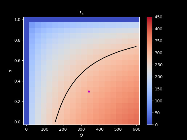
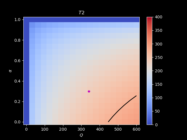
Assume \(\epsilon = 0.586\) (why?) and \(T_{e}=255\) K (why?), we can have
From observations:
Note
The radiative equilibrium solution for the two-layer model is substantially warmer at the surface and colder in the lower troposphere than the real atmosphere.
If we fix \(T_{e} = 255\) K:
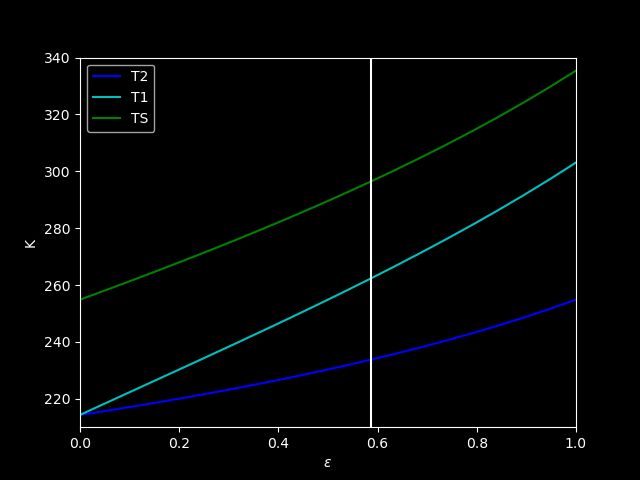
If we fix \(\epsilon=0.586\):
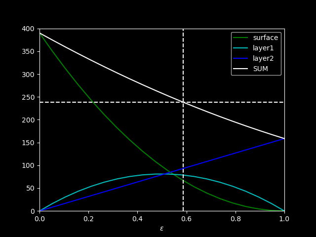
Level of emission#
From above results, we can decompose total OLR to the contributions from each layer:
If we assume \(T_s\)=288 K, \(T_1\)=275 K, \(T_2\)=230 K, and \(\epsilon=0.586\), then we can get:
Radiative forcing#
We define the radiative forcing (\(F_{R}\)) as the change in TOA radiative flux after adding absorbers (not being adjusted by other processes, such as feedbacks). In orther words, the radiative flux change due to changes in atmospheric composition.
where negative value means radiative emission to the space, so the Earth is losing energy, vice versa.
In the two-layer model, the only component that can change due to adding absorbers is OLR. In a more realistic scenasio, the radiative forcing invovles with stratospheric adjustment. Here’s a schematic from Hansen’s 1997 classic paper:
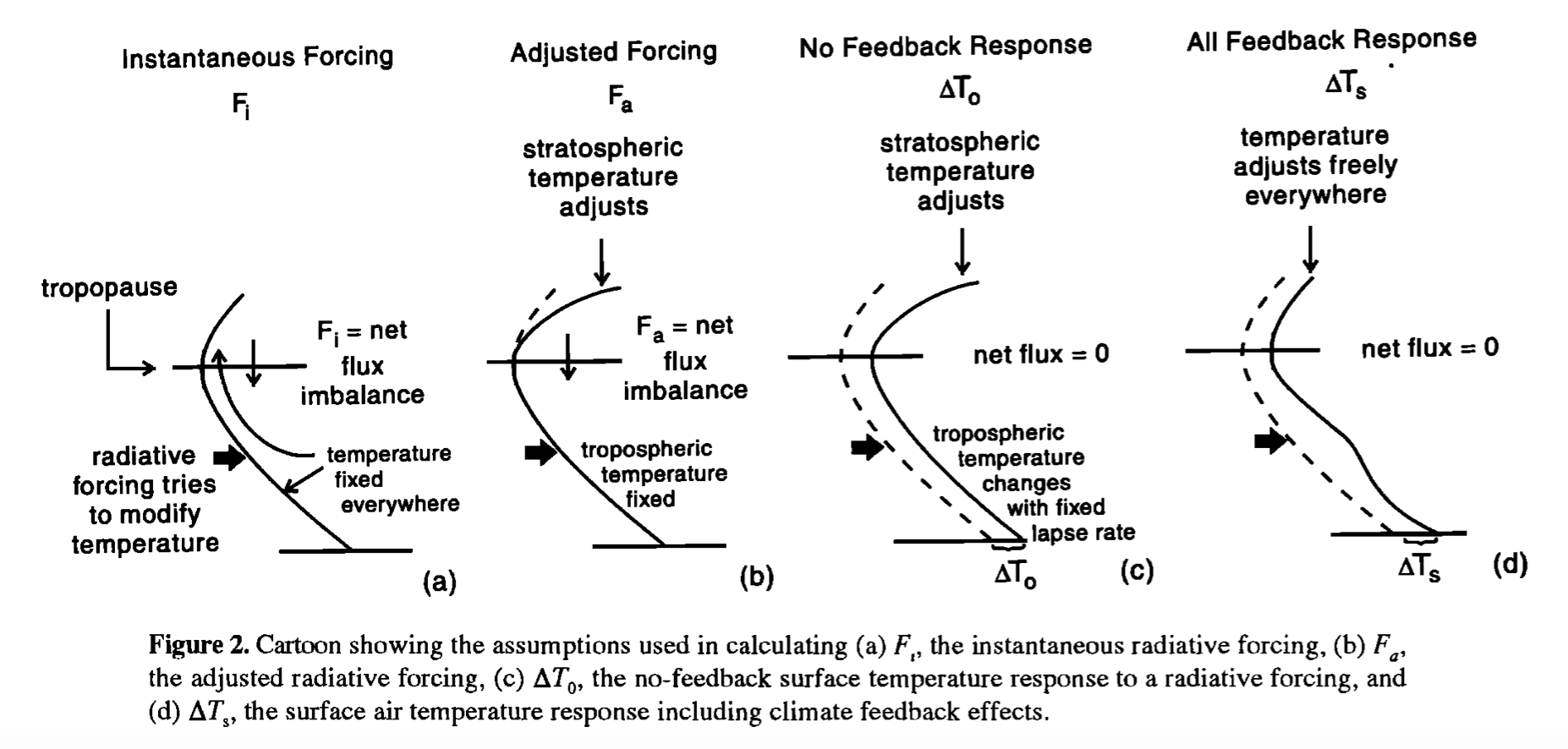
instantaneous radiative forcing
adjusted radiative forcing
effective radiative forcing (???)
Let’s go back to our two-layer model with level of emission (Equation (53)). If we perturb the emmisivity:
The atmospheric temperatures are assumed unchanged, so we can derive:
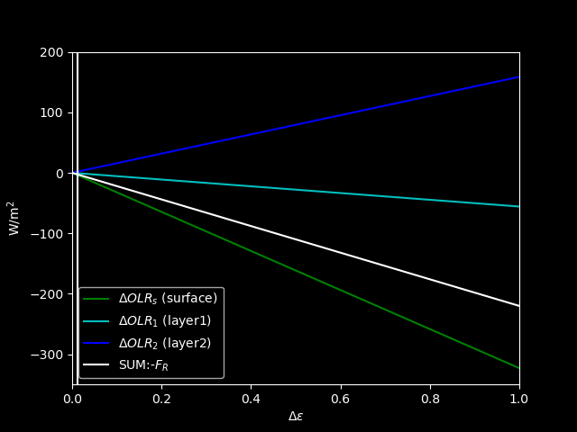
We subtract each term from original value to get “changes” of OLR:
If we ignore high-order term:
What do these results mean?
The radiative forcing then becomes:
Will \(F_R\) be negative or positive? It is complicated and depending on the vertical temperature profile.
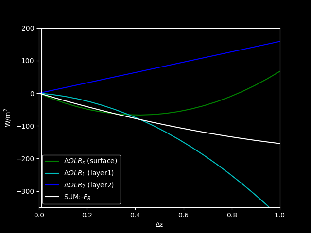
If we fix temepratures from observations:
If we include nonlinear terms:
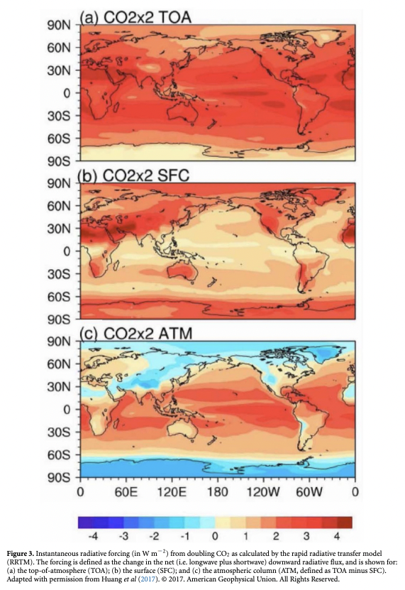
Below is the intantaneous radiative forcing estimated by a rapid radiative transfer model (RRTM) from Previdi et al. (2020):
30-layer model#
We can construct a 30-layer model by hand, but it could be challenging and not feasible. Therefore, it would be useful, and sometimes helpful, to konw climlab, developed by Professor Brian E. J. Rose. Let’s start with a few examples: here. We will see how to construct a 30-layer model, which seems not feasible for solving the equations analytically.
Note
You can find more materials and notes prepared by Professor Brian E. J. Rose: here. They are awesome!!!
We now follow an example from Professor Rose’s notes to demonstrate the results of 30-layer grey-gas model.
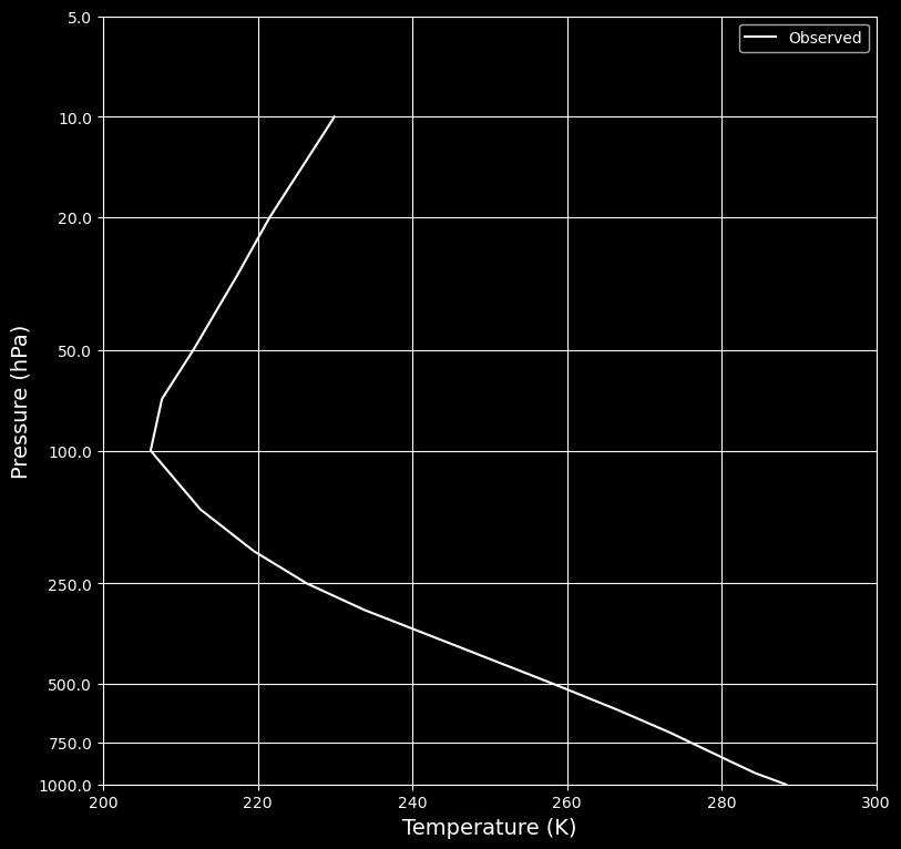
We first look at the observed temperature profile, which we need to specify later in the 30-layer model.
import numpy as np
import matplotlib.pyplot as plt
import xarray as xr
import climlab
from scipy.optimize import brentq

plt.style.use('dark_background')

# read data from ncep reanalysis data
url = 'http://apdrc.soest.hawaii.edu:80/dods/public_data/Reanalysis_Data/NCEP/NCEP/clima/pressure/air'
air = xr.open_dataset(url)
# The name of the vertical axis is different than the NOAA ESRL version..
ncep_air = air.rename({'lev': 'level'})
print('ncep_air')
print(ncep_air)

#  Take global, annual average and convert to Kelvin
weight = np.cos(np.deg2rad(ncep_air.lat)) / np.cos(np.deg2rad(ncep_air.lat)).mean(dim='lat')
Tglobal = (ncep_air.air * weight).mean(dim=('lat','lon','time'))
Tglobal += climlab.constants.tempCtoK
print('Tglobal')
print(Tglobal)


#  A handy re-usable routine for making a plot of the temperature profiles
#  We will plot temperatures with respect to log(pressure) to get a height-like coordinate

def zstar(lev):
    return -np.log(lev / climlab.constants.ps)

def plot_soundings(result_list, name_list, plot_obs=True, fixed_range=True):
    color_cycle=['r', 'g', 'b', 'y']
    # col is either a column model object or a list of column model objects
    #if isinstance(state_list, climlab.Process):
    #    # make a list with a single item
    #    collist = [collist]
    fig, ax = plt.subplots(figsize=(9,9))
    if plot_obs:
        ax.plot(Tglobal, zstar(Tglobal.level), color='w', label='Observed')
    for i, state in enumerate(result_list):
        Tatm = state['Tatm']
        lev = Tatm.domain.axes['lev'].points
        Ts = state['Ts']
        ax.plot(Tatm, zstar(lev), color=color_cycle[i], label=name_list[i])
        ax.plot(Ts, 0, 'o', markersize=12, color=color_cycle[i])
    #ax.invert_yaxis()
    yticks = np.array([1000., 750., 500., 250., 100., 50., 20., 10., 5.])
    ax.set_yticks(-np.log(yticks/1000.))
    ax.set_yticklabels(yticks)
    ax.set_xlabel('Temperature (K)', fontsize=14)
    ax.set_ylabel('Pressure (hPa)', fontsize=14)
    ax.grid()
    ax.legend()
    if fixed_range:
        ax.set_xlim([200, 300])
        ax.set_ylim(zstar(np.array([1000., 5.])))
    #ax2 = ax.twinx()

    return ax

plot_soundings([],[] );
/Users/yuchiaol_ntuas/miniconda3/lib/python3.11/site-packages/xarray/coding/times.py:170: SerializationWarning: Ambiguous reference date string: 1-1-1 00:00:0.0. The first value is assumed to be the year hence will be padded with zeros to remove the ambiguity (the padded reference date string is: 0001-1-1 00:00:0.0). To remove this message, remove the ambiguity by padding your reference date strings with zeros.
  warnings.warn(warning_msg, SerializationWarning)
/Users/yuchiaol_ntuas/miniconda3/lib/python3.11/site-packages/xarray/coding/times.py:995: SerializationWarning: Unable to decode time axis into full numpy.datetime64 objects, continuing using cftime.datetime objects instead, reason: dates out of range
  dtype = _decode_cf_datetime_dtype(data, units, calendar, self.use_cftime)
/Users/yuchiaol_ntuas/miniconda3/lib/python3.11/site-packages/xarray/core/indexing.py:630: SerializationWarning: Unable to decode time axis into full numpy.datetime64 objects, continuing using cftime.datetime objects instead, reason: dates out of range
  array = array.get_duck_array()
/Users/yuchiaol_ntuas/miniconda3/lib/python3.11/site-packages/xarray/core/indexing.py:500: SerializationWarning: Unable to decode time axis into full numpy.datetime64 objects, continuing using cftime.datetime objects instead, reason: dates out of range
  return np.asarray(self.get_duck_array(), dtype=dtype)
ncep_air
<xarray.Dataset> Size: 17MB
Dimensions:         (time: 12, level: 17, lat: 73, lon: 144)
Coordinates:
  * time            (time) object 96B 0001-01-01 00:00:00 ... 0001-12-01 00:0...
  * level           (level) float64 136B 1e+03 925.0 850.0 ... 30.0 20.0 10.0
  * lat             (lat) float64 584B -90.0 -87.5 -85.0 ... 85.0 87.5 90.0
  * lon             (lon) float64 1kB 0.0 2.5 5.0 7.5 ... 352.5 355.0 357.5
Data variables:
    air             (time, level, lat, lon) float32 9MB ...
    valid_yr_count  (time, level, lat, lon) float32 9MB ...
Attributes:
    title:          NMC reanalysis atlas
    Conventions:    COARDS\nGrADS
    dataType:       Grid
    documentation:  http://apdrc.soest.hawaii.edu/datadoc/ncep_clima.php
    history:        Wed Apr 23 10:40:31 HST 2025 : imported by GrADS Data Ser...
Tglobal
<xarray.DataArray (level: 17)> Size: 136B
array([288.32908417, 284.35700336, 280.98832797, 273.36994171,
       266.701657  , 258.26115449, 247.57953059, 233.78031101,
       226.35208723, 219.49775966, 212.5864428 , 206.14394556,
       207.6170672 , 211.66335696, 217.29641375, 221.55605035,
       229.93001391])
Coordinates:
  * level    (level) float64 136B 1e+03 925.0 850.0 700.0 ... 30.0 20.0 10.0
Now we construct our 30-layer model using the observed temperature profile.
# initialize a grey radiation model with 30 levels
col = climlab.GreyRadiationModel()
print('col')
print(col)
# interpolate to 30 evenly spaced pressure levels
lev = col.lev
Tinterp = np.interp(lev, np.flipud(Tglobal.level), np.flipud(Tglobal))
print('Tinterp')
print(Tinterp)
# Need to 'flipud' because the interpolation routine
# needs the pressure data to be in increasing order
# Initialize model with observed temperatures
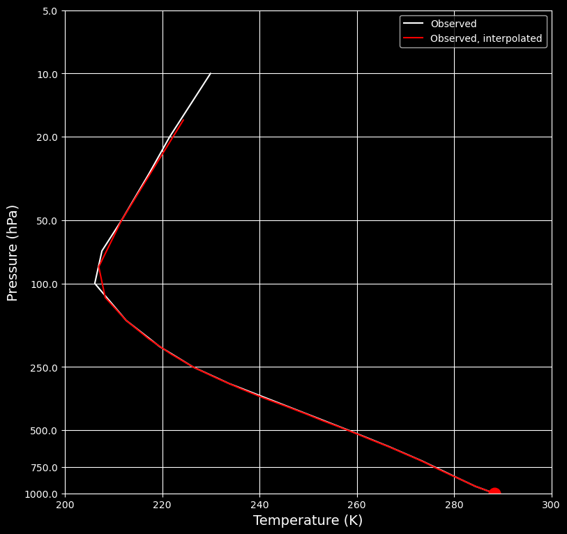
col.Ts[:] = Tglobal[0]
col.Tatm[:] = Tinterp
# This should look just like the observations
result_list = [col.state]
name_list = ['Observed, interpolated']
plot_soundings(result_list, name_list);
col.compute_diagnostics()
print('col.OLR')
print(col.OLR)
# Need to tune absorptivity to get OLR = 238.5
epsarray = np.linspace(0.01, 0.1, 100)
OLRarray = np.zeros_like(epsarray)
for i in range(epsarray.size):
col.subprocess['LW'].absorptivity = epsarray[i]
col.compute_diagnostics()
OLRarray[i] = col.OLR
def OLRanom(eps):
col.subprocess['LW'].absorptivity = eps
col.compute_diagnostics()
return col.OLR - 238.5
# Use numerical root-finding to get the equilibria
# brentq is a root-finding function
# Need to give it a function and two end-points
# It will look for a zero of the function between those end-points
eps = brentq(OLRanom, 0.01, 0.1)
print('eps')
print(eps)
col.subprocess.LW.absorptivity = eps
print('col.subprocess.LW.absorptivity')
print(col.subprocess.LW.absorptivity)
col.compute_diagnostics()
print('col.OLR')
print(col.OLR)
col
climlab Process of type <class 'climlab.model.column.GreyRadiationModel'>.
State variables and domain shapes:
  Ts: (1,)
  Tatm: (30,)
The subprocess tree:
Untitled: <class 'climlab.model.column.GreyRadiationModel'>
   LW: <class 'climlab.radiation.greygas.GreyGas'>
   SW: <class 'climlab.radiation.greygas.GreyGasSW'>
   insolation: <class 'climlab.radiation.insolation.FixedInsolation'>

Tinterp
[224.34737153 211.66335696 206.96234647 208.29144464 212.5864428
 217.19398737 221.78253551 226.35208723 231.30423641 236.08018094
 240.6799208  245.27966066 249.35980124 252.92034254 256.48088384
 259.66790491 262.48140575 265.29490658 267.81303779 270.03579936
 272.25856092 274.21642907 275.90940379 277.60237852 279.29535324
 280.98832797 282.48551703 283.98270609 285.6810303  287.44639955]
col.OLR
[263.15004222]
eps
0.053690752586678596
col.subprocess.LW.absorptivity
[0.05369075 0.05369075 0.05369075 0.05369075 0.05369075 0.05369075
 0.05369075 0.05369075 0.05369075 0.05369075 0.05369075 0.05369075
 0.05369075 0.05369075 0.05369075 0.05369075 0.05369075 0.05369075
 0.05369075 0.05369075 0.05369075 0.05369075 0.05369075 0.05369075
 0.05369075 0.05369075 0.05369075 0.05369075 0.05369075 0.05369075]
col.OLR
[238.5]
We now calculate the radiative forcing.
#  clone our model using a built-in climlab function
col2 = climlab.process_like(col)
print('col2')
print(col2)

col2.subprocess['LW'].absorptivity *= 1.02
print(col2.subprocess['LW'].absorptivity)

#  Radiative forcing by definition is the change in TOA radiative flux,
# HOLDING THE TEMPERATURES FIXED.
print('col2.Ts - col.Ts')
print(col2.Ts - col.Ts)

col2.compute_diagnostics()
print('col2.OLR')
print(col2.OLR)

RF = -(col2.OLR - col.OLR)
print( 'The radiative forcing is %.2f W/m2.' %RF)
col2
climlab Process of type <class 'climlab.model.column.GreyRadiationModel'>.
State variables and domain shapes:
  Ts: (1,)
  Tatm: (30,)
The subprocess tree:
Untitled: <class 'climlab.model.column.GreyRadiationModel'>
   LW: <class 'climlab.radiation.greygas.GreyGas'>
   SW: <class 'climlab.radiation.greygas.GreyGasSW'>
   insolation: <class 'climlab.radiation.insolation.FixedInsolation'>

[0.05476457 0.05476457 0.05476457 0.05476457 0.05476457 0.05476457
 0.05476457 0.05476457 0.05476457 0.05476457 0.05476457 0.05476457
 0.05476457 0.05476457 0.05476457 0.05476457 0.05476457 0.05476457
 0.05476457 0.05476457 0.05476457 0.05476457 0.05476457 0.05476457
 0.05476457 0.05476457 0.05476457 0.05476457 0.05476457 0.05476457]
col2.Ts - col.Ts
[0.]
col2.OLR
[236.65384095]
The radiative forcing is 1.85 W/m2.
Finally, we calculate the radiative equilibrium state:
re = climlab.process_like(col)
#  To get to equilibrium, we just time-step the model forward long enough
re.integrate_years(1.)

#  Check for energy balance
print( 'The net downward radiative flux at TOA is %.4f W/m2.' %(re.ASR - re.OLR))

result_list.append(re.state)
name_list.append('Radiative equilibrium (grey gas)')
plot_soundings(result_list, name_list)
Integrating for 365 steps, 365.2422 days, or 1.0 years.
Total elapsed time is 0.9993368783782377 years.
The net downward radiative flux at TOA is -0.0015 W/m2.
<Axes: xlabel='Temperature (K)', ylabel='Pressure (hPa)'>
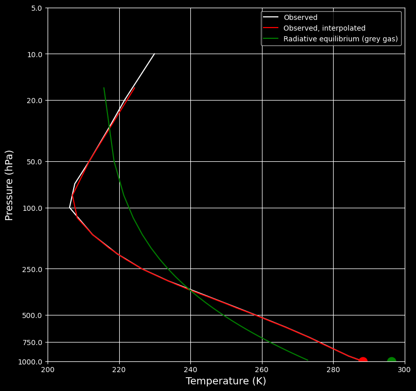
What do you find?
Homework assignment 2 (due xxx)#
Given an observational vertical temperature profile (\(T_s\)=288 K, \(T_1\)=275 K, \(T_2\)=230 K, and OLR=238.5 \(\mbox{W/m}^2\), could you find the value for \(\epsilon\)?
What is the radiative forcing \(R\) in an isothermal atmosphere? Please use the two-layer model to support your guess.
Assume we add greenhouse gases into the atmopshere with observed temperatures, that is:\(\Delta \epsilon = 0.02\times \epsilon\). What is the radiative forcing? Be sure you understand the sign.
Can you add convective adjustment and ozone into your 30-layer model?
Final project 2#
Could you construct a n-layer model, for n>4? Please discuss:
The upward and downward longwave beams, and the level of emission.
What are the atmospheric temperatures in each layer? And what is the sufrave temperature?
If you add greenhouse gases, what are the temperatures change?
What is the radiative forcing in each layer? How does it change when the emmisivity increases?
Final project 3#
Could you include seasonal and latitudinal variation of ozone in your 30-layer model? Please discuss the aspects discussed above.