12. Climate Sensitivity and Feedback#
Radiative forcing#
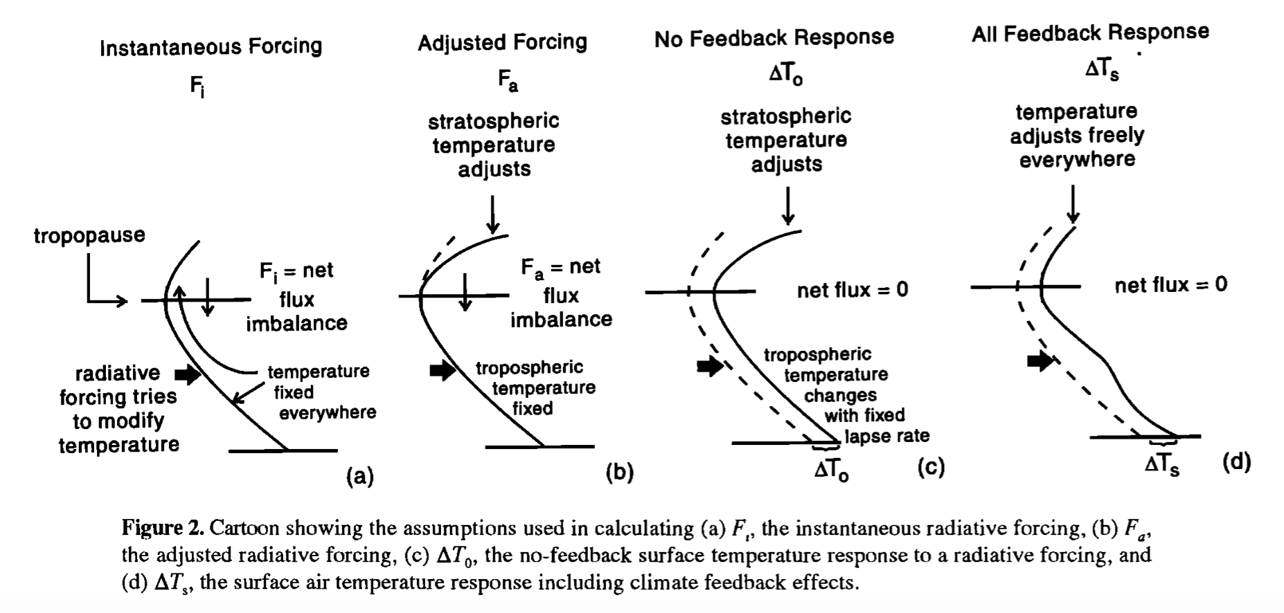
We start with the radiative forcing in a RCE model. Recall that the instantaneous radiative forcing is the quick change in the TOA energy budget before the climate system begins to adjust.
If we consider the forcing as doubling CO2, we could write the radiative forcing as:
What is happening after we add more CO2 in the atmosphere?
The atmosphere is less efficient at radiating energy away to space (reducing emissivity, right?).
OLR will decrease
The climate system will begin gaining energy.
Now let’s build a RCE model and analyze its radiative forcing.
#  This code is used just to create the skew-T plot of global, annual mean air temperature
%matplotlib inline
import numpy as np
import matplotlib.pyplot as plt
import xarray as xr
from metpy.plots import SkewT
import climlab

#plt.style.use('dark_background')

#  This code is used just to create the skew-T plot of global, annual mean air temperature
#ncep_url = "http://www.esrl.noaa.gov/psd/thredds/dodsC/Datasets/ncep.reanalysis.derived/"
ncep_url = "/Users/yuchiaol_ntuas/Desktop/ebooks/data/"
#time_coder = xr.coders.CFDatetimeCoder(use_cftime=True)
ncep_air = xr.open_dataset( ncep_url + "air.mon.1981-2010.ltm.nc", use_cftime=True)
#  Take global, annual average
coslat = np.cos(np.deg2rad(ncep_air.lat))
weight = coslat / coslat.mean(dim='lat')
Tglobal = (ncep_air.air * weight).mean(dim=('lat','lon','time'))

print(Tglobal)

#  Resuable function to plot the temperature data on a Skew-T chart
def make_skewT():
    fig = plt.figure(figsize=(9, 9))
    skew = SkewT(fig, rotation=30)
    skew.plot(Tglobal.level, Tglobal, color='black', linestyle='-', linewidth=2, label='Observations')
    skew.ax.set_ylim(1050, 10)
    skew.ax.set_xlim(-90, 45)
    # Add the relevant special lines
    skew.plot_dry_adiabats(linewidth=0.5)
    skew.plot_moist_adiabats(linewidth=0.5)
    #skew.plot_mixing_lines()
    skew.ax.legend()
    skew.ax.set_xlabel('Temperature (degC)', fontsize=14)
    skew.ax.set_ylabel('Pressure (hPa)', fontsize=14)
    return skew

#  and a function to add extra profiles to this chart
def add_profile(skew, model, linestyle='-', color=None):
    line = skew.plot(model.lev, model.Tatm - climlab.constants.tempCtoK,
             label=model.name, linewidth=2)[0]
    skew.plot(1000, model.Ts - climlab.constants.tempCtoK, 'o',
              markersize=8, color=line.get_color())
    skew.ax.legend()
<xarray.DataArray (level: 17)> Size: 68B
array([ 15.179084  ,  11.207003  ,   7.8383274 ,   0.21994135,
        -6.4483433 , -14.888848  , -25.570469  , -39.36969   ,
       -46.797905  , -53.652245  , -60.56356   , -67.006065  ,
       -65.53293   , -61.48664   , -55.853584  , -51.593952  ,
       -43.21999   ], dtype=float32)
Coordinates:
  * level    (level) float32 68B 1e+03 925.0 850.0 700.0 ... 50.0 30.0 20.0 10.0
# Get the water vapor data from CESM output
#cesm_data_path = "http://thredds.atmos.albany.edu:8080/thredds/dodsC/CESMA/"
cesm_data_path = "/Users/yuchiaol_ntuas/Desktop/ebooks/data/"
atm_control = xr.open_dataset(cesm_data_path + "cpl_1850_f19.cam.h0.nc")
# Take global, annual average of the specific humidity
weight_factor = atm_control.gw / atm_control.gw.mean(dim='lat')
Qglobal = (atm_control.Q * weight_factor).mean(dim=('lat','lon','time'))

#  Make a model on same vertical domain as the GCM
mystate = climlab.column_state(lev=Qglobal.lev, water_depth=2.5)
#  Build the radiation model -- just like we already did
rad = climlab.radiation.RRTMG(name='Radiation',
                              state=mystate,
                              specific_humidity=Qglobal.values,
                              timestep = climlab.constants.seconds_per_day,
                              albedo = 0.25,  # surface albedo, tuned to give reasonable ASR for reference cloud-free model
                             )
#  Now create the convection model
conv = climlab.convection.ConvectiveAdjustment(name='Convection',
                                               state=mystate,
                                               adj_lapse_rate=6.5,
                                               timestep=rad.timestep,
                                              )
#  Here is where we build the model by coupling together the two components
rcm = climlab.couple([rad, conv], name='Radiative-Convective Model')

print(rcm)

print(rcm.subprocess['Radiation'].absorber_vmr['CO2'])

print(rcm.integrate_years(5))

print(rcm.ASR - rcm.OLR)
climlab Process of type <class 'climlab.process.time_dependent_process.TimeDependentProcess'>.
State variables and domain shapes:
  Ts: (1,)
  Tatm: (26,)
The subprocess tree:
Radiative-Convective Model: <class 'climlab.process.time_dependent_process.TimeDependentProcess'>
   Radiation: <class 'climlab.radiation.rrtm.rrtmg.RRTMG'>
      SW: <class 'climlab.radiation.rrtm.rrtmg_sw.RRTMG_SW'>
      LW: <class 'climlab.radiation.rrtm.rrtmg_lw.RRTMG_LW'>
   Convection: <class 'climlab.convection.convadj.ConvectiveAdjustment'>

0.000348
Integrating for 1826 steps, 1826.2110000000002 days, or 5 years.
Total elapsed time is 4.999422301147019 years.
None
[-3.3651304e-11]
Now we make another RCE model with CO2 doubled!
# Make an exact clone with same temperatures
rcm_2xCO2 = climlab.process_like(rcm)
rcm_2xCO2.name = 'Radiative-Convective Model (2xCO2 initial)'

#  Check to see that we indeed have the same CO2 amount
print(rcm_2xCO2.subprocess['Radiation'].absorber_vmr['CO2'])

#  Now double it!
rcm_2xCO2.subprocess['Radiation'].absorber_vmr['CO2'] *= 2

print(rcm_2xCO2.subprocess['Radiation'].absorber_vmr['CO2'])
0.000348
0.000696
Let’s quickly check the instantaneous radiative forcing:
rcm_2xCO2.compute_diagnostics()

print(rcm_2xCO2.ASR - rcm.ASR)

print(rcm_2xCO2.OLR - rcm.OLR)

DeltaR_instant = (rcm_2xCO2.ASR - rcm_2xCO2.OLR) - (rcm.ASR - rcm.OLR)

print(DeltaR_instant)
[0.06274162]
[-2.11458541]
[2.17732704]
What is the instantaneous radiative forcing in our two/three-layer model?
Now we briefly calculate the adjusted radiative forcing. Recall that the adjusted radiative forcing is that the stratosphere is adjusted while the troposphere does not.
# print out troposphere
print(rcm.lev[13:])

rcm_2xCO2_strat = climlab.process_like(rcm_2xCO2)
rcm_2xCO2_strat.name = 'Radiative-Convective Model (2xCO2 stratosphere-adjusted)'
for n in range(1000):
    rcm_2xCO2_strat.step_forward()
# hold tropospheric and surface temperatures fixed
    rcm_2xCO2_strat.Tatm[13:] = rcm.Tatm[13:]
    rcm_2xCO2_strat.Ts[:] = rcm.Ts[:]

DeltaR = (rcm_2xCO2_strat.ASR - rcm_2xCO2_strat.OLR) - (rcm.ASR - rcm.OLR)
print(DeltaR)
[226.513265 266.481155 313.501265 368.81798  433.895225 510.455255
 600.5242   696.79629  787.70206  867.16076  929.648875 970.55483
 992.5561  ]
[4.28837377]
Radiative forcing gives us some insights about how the changes of forcing could tranfer energy to the system, and temperature might change. But not the final temperature reaching equilibrium.
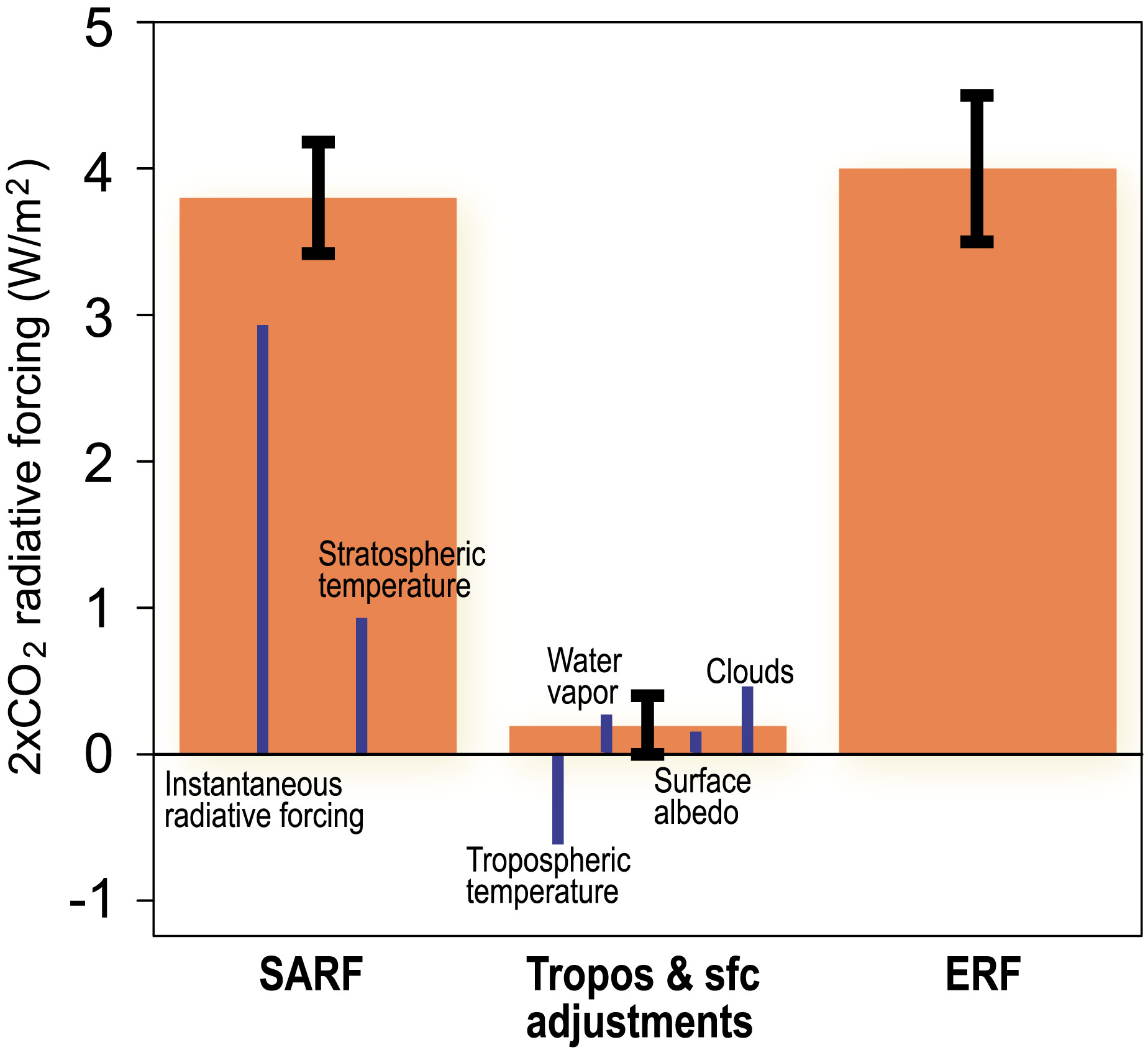
Sherwood et al. (2020) summarize the radiative forcing:
Equilibrium climate sensitivity (ECS) without feedback#
We define the ECS as “The global mean surface warming necessary to balance the planetary energy budget after a doubling of atmospheric CO2”.
If we assume incoming shortwave radiation does not change (e.g., the planetary albedo does not change) after doubling CO2, the climate system has to adjust to new equilibrium temperature. This new temperature must balance the radiative forcing. So, we can get:
where \(OLR_{f}\) is the equilibrated \(OLR\) associated with the new qeuilibrium temperature.
We know that from our zero-dimensional energy-balance model, we derive the OLR sensitivity to temperature change:
So we can write:
The energy balance gives us:
Assume the actual radiative forcing after doubling CO2 is about 4 W/m\(^2\)/K, we can get:
This is the ECS without feedback using zero-dimensional model!!!
OLRobserved = 238.5  # in W/m2
sigma = 5.67E-8  # S-B constant
Tsobserved = 288.  # global average surface temperature
tau = OLRobserved / sigma / Tsobserved**4  # solve for tuned value of transmissivity

lambda_0 = 4 * sigma * tau * Tsobserved**3

DeltaR_test = 4.  # Radiative forcing in W/m2
DeltaT0 = DeltaR_test / lambda_0
print( 'The Equilibrium Climate Sensitivity in the absence of feedback is {:.1f} K.'.format(DeltaT0))
The Equilibrium Climate Sensitivity in the absence of feedback is 1.2 K.
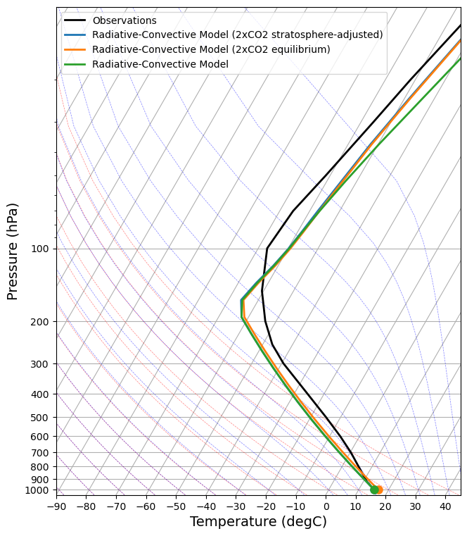
Now we use RCE models to estimate ECS.
rcm_2xCO2_eq = climlab.process_like(rcm_2xCO2_strat)
rcm_2xCO2_eq.name = 'Radiative-Convective Model (2xCO2 equilibrium)'
rcm_2xCO2_eq.integrate_years(5)
print('rcm_2xCO2_eq.ASR - rcm_2xCO2_eq.OLR')
print(rcm_2xCO2_eq.ASR - rcm_2xCO2_eq.OLR)
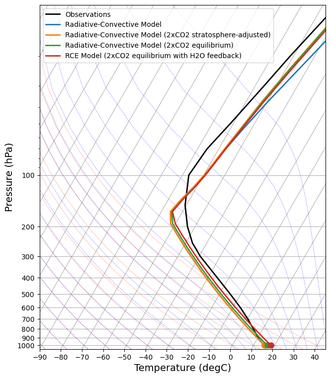
skew = make_skewT()
add_profile(skew, rcm_2xCO2_strat)
add_profile(skew, rcm_2xCO2_eq)
add_profile(skew, rcm)
ECS_nofeedback = rcm_2xCO2_eq.Ts - rcm.Ts
print('ECS with no feedback')
print(ECS_nofeedback)
print('rcm_2xCO2_eq.OLR - rcm.OLR')
print(rcm_2xCO2_eq.OLR - rcm.OLR)
print('rcm_2xCO2_eq.ASR - rcm.ASR')
print(rcm_2xCO2_eq.ASR - rcm.ASR)
lambda0 = DeltaR / ECS_nofeedback
print('lambda0')
print(lambda0)
Integrating for 1826 steps, 1826.2110000000002 days, or 5 years.
Total elapsed time is 12.736753858124827 years.
rcm_2xCO2_eq.ASR - rcm_2xCO2_eq.OLR
[1.31308298e-11]
ECS with no feedback
[1.29984831]
rcm_2xCO2_eq.OLR - rcm.OLR
[0.05080282]
rcm_2xCO2_eq.ASR - rcm.ASR
[0.05080282]
lambda0
[3.29913401]
Climate feedback#
I guess that the feedback concept is inherited from electronic engineering. For example, Professor Gu-Yeon Wei’s lecture 18 introduced the feedback concept (here):
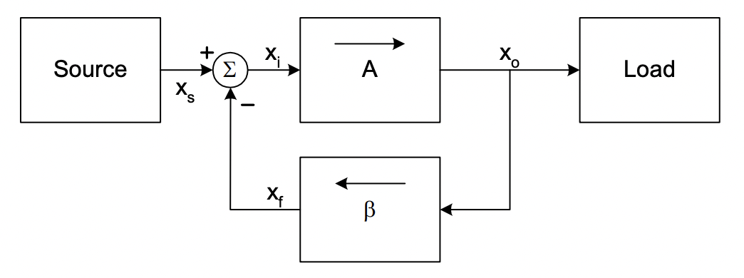
In climate science, we can think of “Source” as forcing or input added to the system, A as the whole process in the system, \(\beta\) (gain) as the amplifier or deamplifier, and the load is the output.
We use \(f\) to quantify the effect and strength of \(\beta\) (gain). If it is positive (\(f>0\)), we call it amplifying feedback. If it is negative (\(f<0\)), we call it dampling feedback.
Can you give examples for positive and negative feedbacks in the atmosphere or climate system?
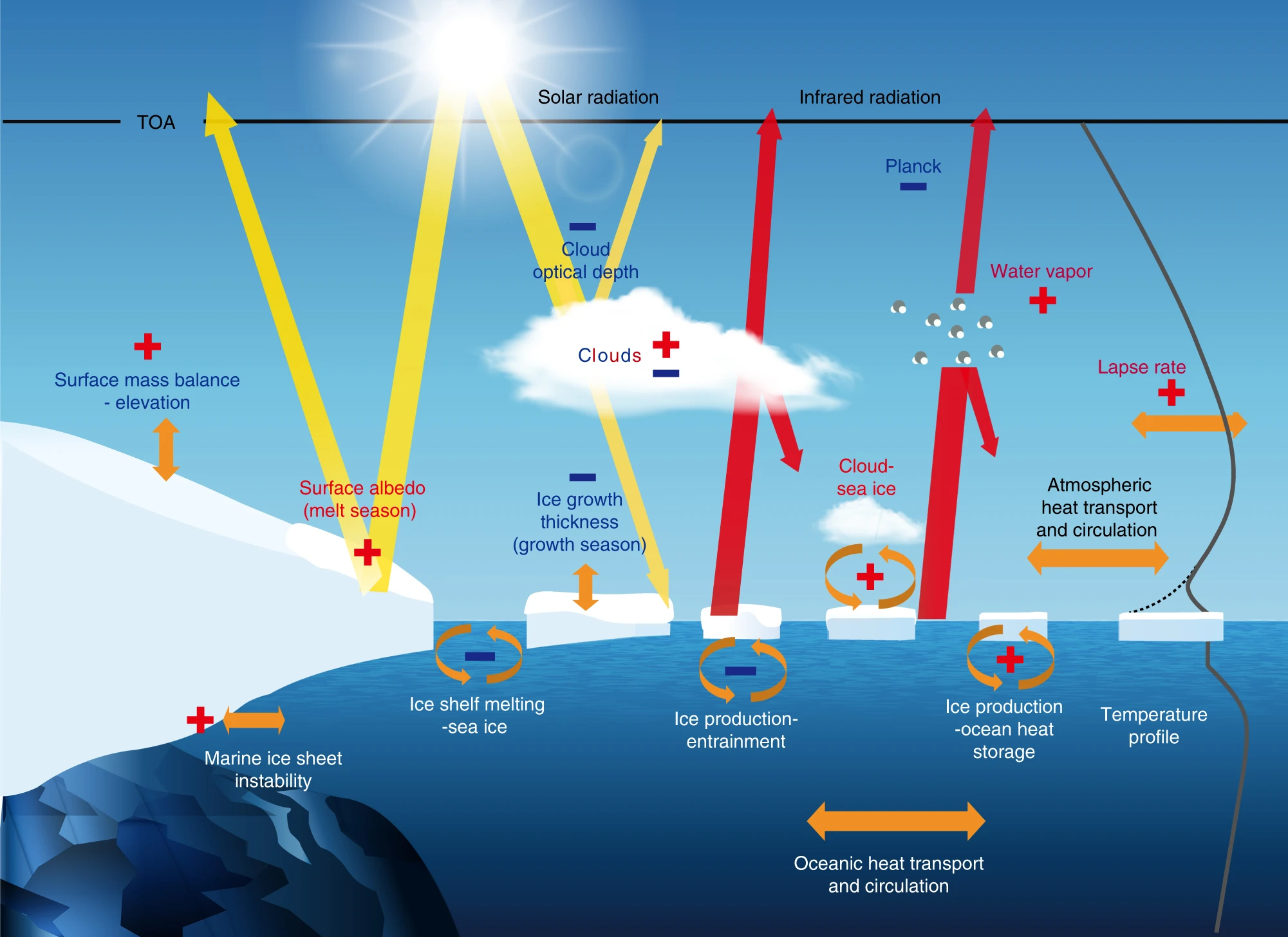
In Arctic climate system, the feedbacks could be complex. In Goosse et al. (2018), they summarized some feedbacks in the Arctic:
Let’s work on how to quantify the effect of feedbacks. We strat with the temperature change considered in a system without feedback:
We assume that a positive feedback (e.g., water vapor feedback) is included and taking action. So its effect is to “enhance” the temperature change positively with a fraction of \(f\):
Note
With infinity loops, we take the sum of each feedback effect:
Sum the original response to forcing \(\Delta R = \lambda_{0}\Delta T_{0}\),
So the final response is
We define the gain as:
What does this mean? How about a negative feedback?
If the system has N individual feedbacks, the total effect can be summed:
The ECS now becomes:
We can define feedback parameter in the unit of W/m\(^2\)/K as:
Then:
So the total feedback (parameter) could be decompose into:
Note
\(\lambda_{0}=3.3\) W/m\(^2\)/K is the Planck feedback parameter. This is not a real feedback (right?), and simply as a consequence of a warmer world emits more longwave radiation than a colder world.
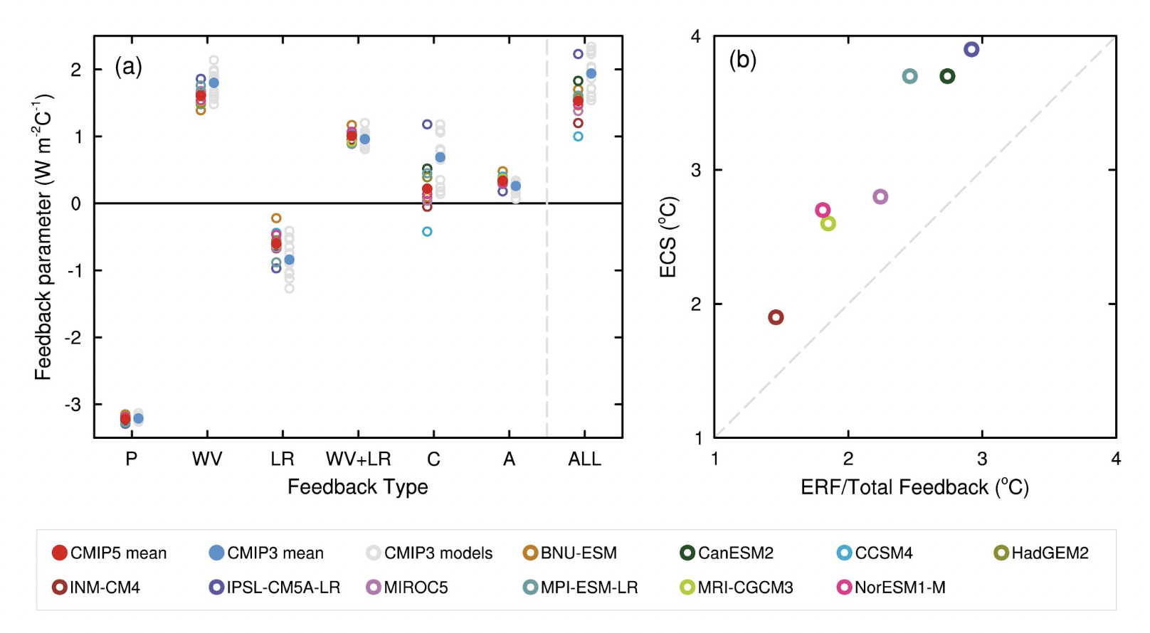
This formulation is very useful, becasue we can qunatitatively compare the importance of each feedback. Below is an example from my paper:
Now let’s add a water vapor feedback into our RCE model and calculate ECS and feedback parameter.
#  actual specific humidity
q = rcm.subprocess['Radiation'].specific_humidity
#  saturation specific humidity (a function of temperature and pressure)
qsat = climlab.utils.thermo.qsat(rcm.Tatm, rcm.lev)
#  Relative humidity
rh = q/qsat

#  Plot relative humidity in percent
fig,ax = plt.subplots()
ax.plot(q*1000, rcm.lev, 'b-')
ax.invert_yaxis()
ax.grid()
ax.set_ylabel('Pressure (hPa)')
ax.set_xlabel('Specific humidity (g/kg)', color='b')
ax.tick_params('x', colors='b')
ax2 = ax.twiny()
ax2.plot(rh*100., rcm.lev, 'r-')
ax2.set_xlabel('Relative humidity (%)', color='r')
ax2.tick_params('x', colors='r')
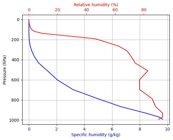
We consider the relative humidity somewhat fixed, while saturation specific humidity varied with temperature changes.
rcm_2xCO2_h2o = climlab.process_like(rcm_2xCO2)
rcm_2xCO2_h2o.name = 'RCE Model (2xCO2 equilibrium with H2O feedback)'

for n in range(2000):
    # At every timestep
    # we calculate the new saturation specific humidity for the new temperature
    #  and change the water vapor in the radiation model
    #  so that relative humidity is always the same
    qsat = climlab.utils.thermo.qsat(rcm_2xCO2_h2o.Tatm, rcm_2xCO2_h2o.lev)
    rcm_2xCO2_h2o.subprocess['Radiation'].specific_humidity[:] = rh * qsat
    rcm_2xCO2_h2o.step_forward()

# Check for energy balance
print(rcm_2xCO2_h2o.ASR - rcm_2xCO2_h2o.OLR)

skew = make_skewT()
add_profile(skew, rcm)
add_profile(skew, rcm_2xCO2_strat)
add_profile(skew, rcm_2xCO2_eq)
add_profile(skew, rcm_2xCO2_h2o)
[-1.73180638e-07]
ECS = rcm_2xCO2_h2o.Ts - rcm.Ts
print('ECS')
print(ECS)

g = ECS / ECS_nofeedback
print('gain')
print(g)

lambda_net = DeltaR / ECS
print('lambda_net')
print(lambda_net)

print('lambda0')
print(lambda0)

lambda_h2o = lambda0 - lambda_net
print('lambda_h2o')
print(lambda_h2o)
ECS
[2.98902357]
gain
[2.29951722]
lambda_net
[1.43470724]
lambda0
[3.29913401]
lambda_h2o
[1.86442677]
“For every 1 degree of surface warming, the increased water vapor greenhouse effect provides an additional 1.86 W m\(^{-2}\) of radiative forcing.”
Flato et al. (2013) in IPCC AR5 reported the climate feedbacks:
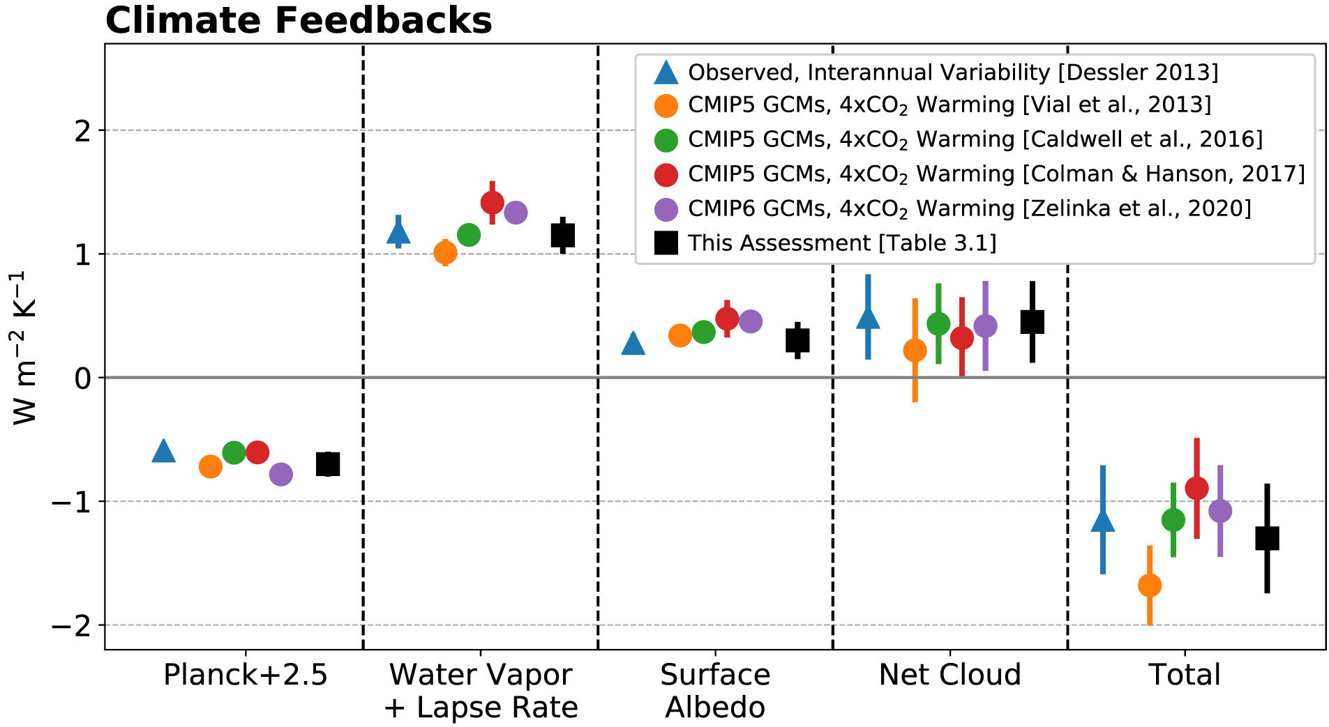
Sherwood et al. (2020) summarize the climate feedbacks:
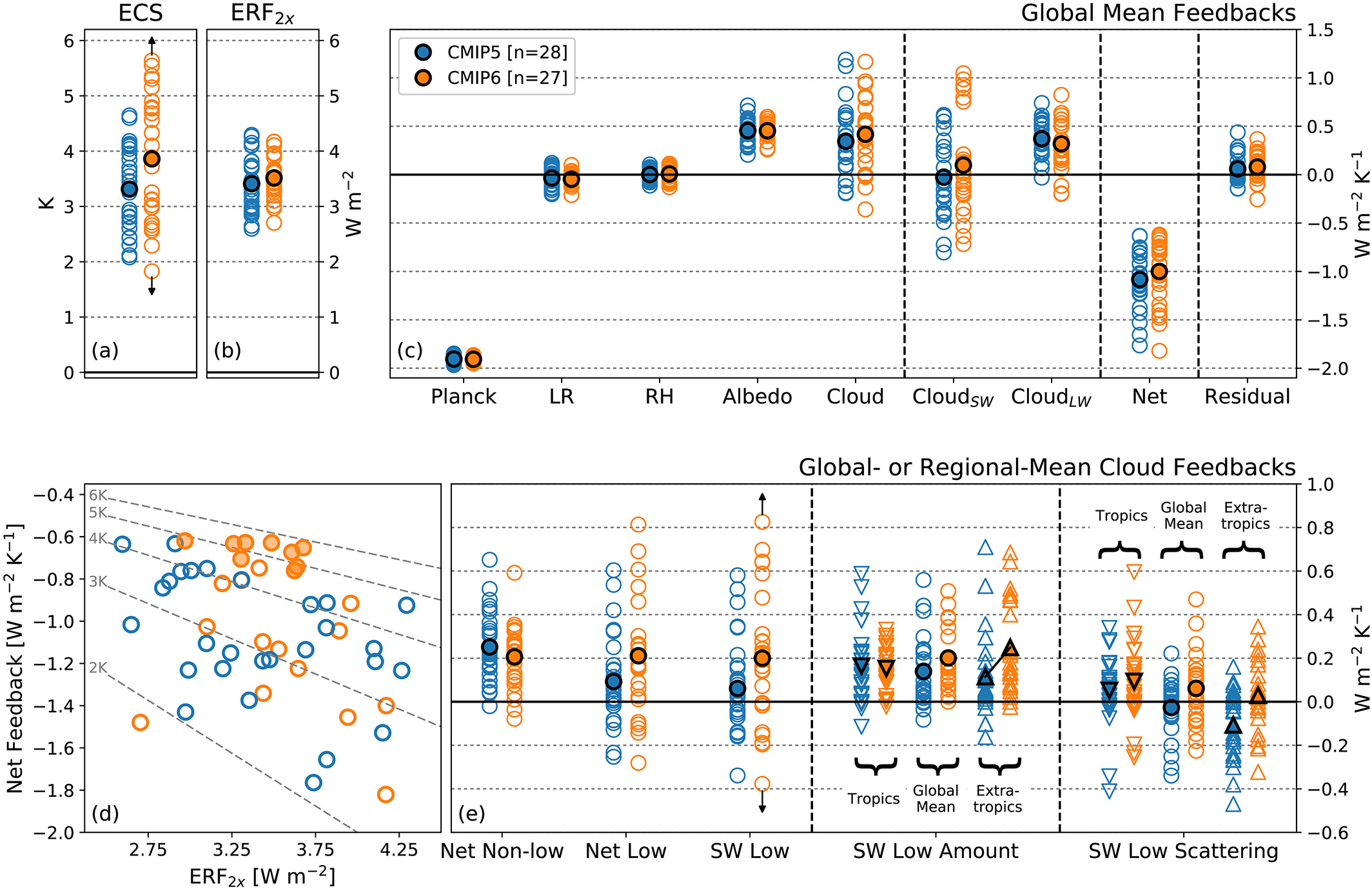
Zelinka et a. (2020) highlighted the uncertainty of ECS comes from the uncertainty of cloud feedback:
The physical model - putting together#
We review Section 2.2 of Sherwood et al. (2020) to put everything together. This is the conventional model for feedback-forcing theory.
where \(\Delta N\) is the net downward radiation imbalance at TOA, \(\Delta F\) is the radiative forcing, and \(\Delta R\) is the radiative response due to direct or indirect changes in temperature, and \(V\) is the unrelated processes.
Assume that the radiative response \(\Delta R\) is proportional to first order of the forced change in global mean surface air temperature (\(\Delta T_s\), using Taylor expansion), we can get:
Note
What is the sign of \(\lambda\)? Can the system reach to an equilibrium state if \(\lambda\) is positive?
Consider the climate system reaches an equilibrium state over a sufficient long time, so we can neglect \(\Delta N\) and \(V\).
So the climate sensitivity of doubling CO2 can be expressed as below:
The feedback \(\lambda\) can be decomposed into each feedback process:
Feebacks can change strength in different climate state –> state dependence \(\Delta \lambda_{state}\)
\(\Delta N\) can not only depend on global-mean surface air temperature but also the geographic distribution or pattern –> pattern effect \(\Delta \lambda_{pattern}\)
We can modify the model as:
where
How to calculate \(\Delta \lambda_{state}\) and \(\Delta \lambda_{pattern}\) is another long story.
Radiative kernel analysis#
The feedback may/should have spatial structure, right? For example, sea-ice albedo feedback should be strongest in polar regions, but very week or no effect in the tropics, right?
To the end of complex climate model similations, climate scientists have developed a method to compute the feedback with spatial structure. This is called the radiative kernel method.
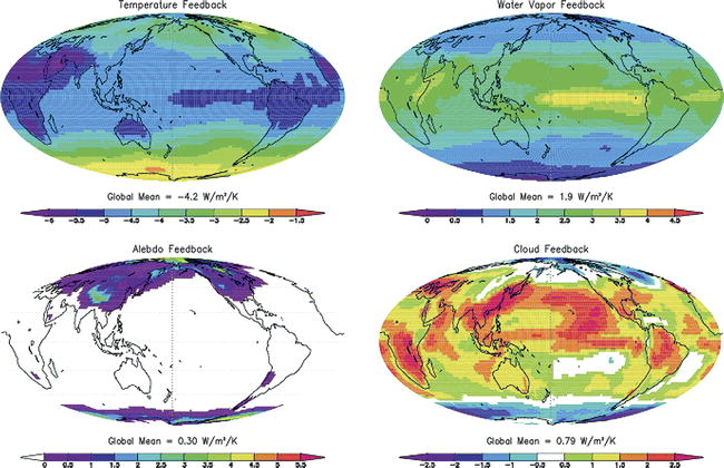
Fig. 45 Multimodel ensemble-mean maps of the temperature, water vapor, albedo, and cloud feedback computed using climate response patterns from the IPCC AR4 models and the GFDL radiative kernels. Source: Soden et al. (2008)#
We use CESM1-CAM5 kernel for demonstration: see Pendergrass et al. (2018).
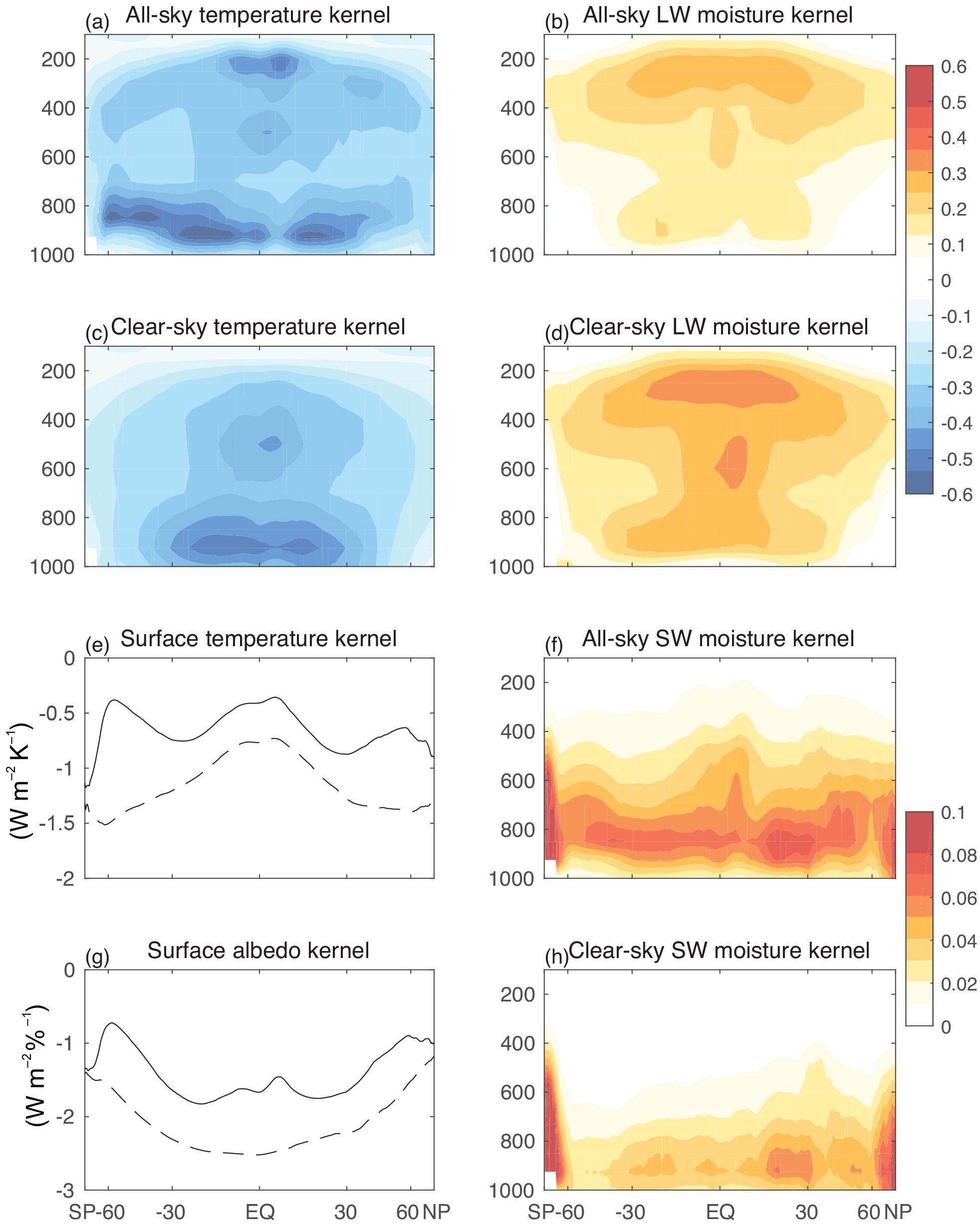
Fig. 46 Top-of-atmosphere kernels from CESM1(CAM5). Zonal, annual-mean temperature, longwave moisture, and shortwave moisture kernels for all-sky and clear-sky. In panels (e) and (g) all-sky kernels are shown in solid lines and clear-sky kernels in dashed lines. The sign convention is positive downward. Source: Pendergrass et al. (2018).#
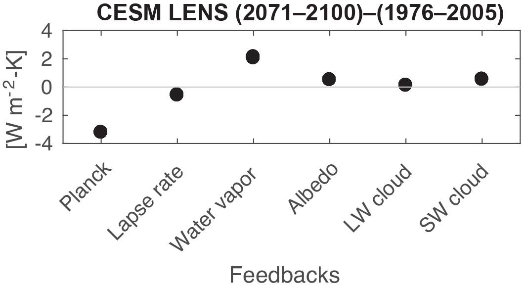
Fig. 47 CESM large-ensemble kernels. Feedback calculation for the CESM 40-member large ensemble using the TOA kernels. Source: Pendergrass et al. (2018).#
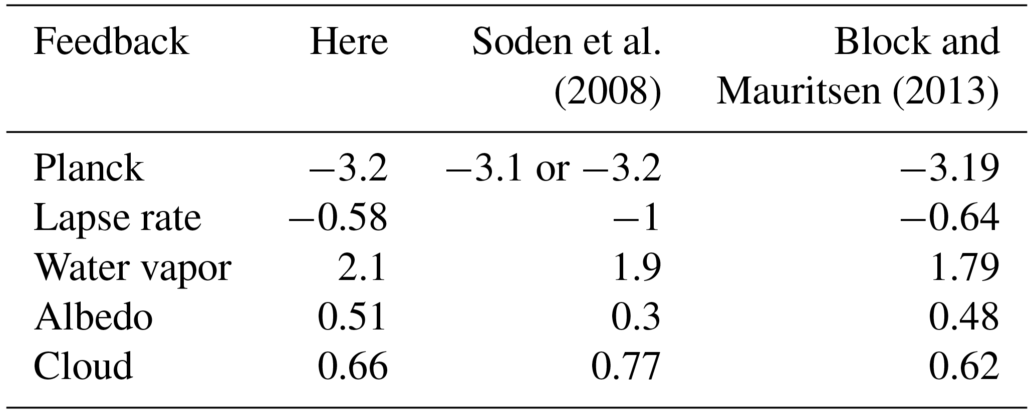
Fig. 48 Comparison of TOA radiative feedbacks. TOA radiative feedbacks (Wm\(^{-2}\) K\(^{-1}\)) averaged over 40 CESM large-ensemble simulations diagnosed with CAM5 radiative kernels, compared against those from CMIP3 model simulations diagnosed with three different kernels as reported by Soden et al. (2008), and MPI-ESM-LR control state kernels and years 21–150 of abrupt carbon dioxide quadrupling simulations from the same model (Block and Mauritsen, 2013). Table from Pendergrass et al. (2018).#
Now let’s try to calculate the feedback parameters and the contributions to temperature responses using CESM1-CAM5 kernel and the data provided.
Note
CESM1-CAM5 kernel can be found on Professor Angeline G. Pendergrass’ GitHub.
Data simulated by CESM1-CAM5 can be found here.
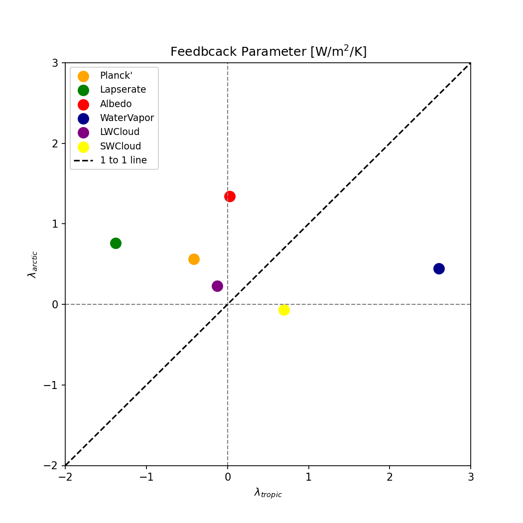
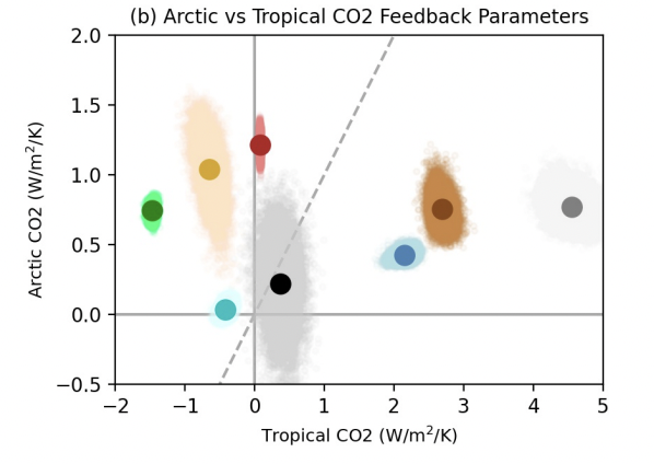
Fig. 49 Feedback parameters to demonstrate Arctic amplification. Credit to 孫翊麒#
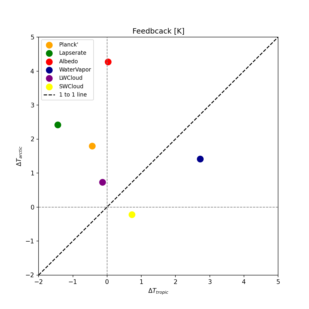
Fig. 50 Temperature responses contributed from Feedbacks to demonstrate Arctic amplification. Credit to 孫翊麒#
Transient and equilibrium responses#
Professor Brian E. J. Rose ran two sets of simulations:
Fully-coupled simulations
pre-industrial control simulation
1% per year CO2 ramp simulation
Slab ocean simulations
pre-industrial control with prescribed q-flux
2xCO2 scenario run out to equilibrium
Which one is the slab ocean model?
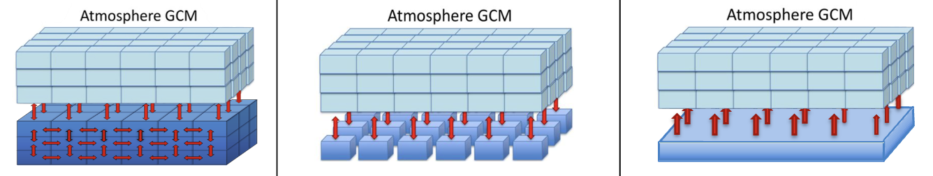
Fig. 51 Figure credit to Ya-Fan Chung.#
We are going to calcualte ECS and transient climate response (TCR). TCR is always smaller than ECS due to the transient effects of ocean heat uptake (?).
Note
The transient climate response (TCR) is defined as the change in global and annual mean surface temperature from an experiment in which the CO2 concentration is increased by 1% yr, and calculated using the difference between the start of the experiment and a 20-year period centred on the time of CO2 doubling.
startingamount = 1.
amount = startingamount
for n in range(70):
    amount *= 1.01
print(amount)
2.006763368395386
What do you find?
%matplotlib inline
import numpy as np
import matplotlib.pyplot as plt
import xarray as xr

casenames = {'cpl_control': 'cpl_1850_f19',
             'cpl_CO2ramp': 'cpl_CO2ramp_f19',
             'som_control': 'som_1850_f19',
             'som_2xCO2':   'som_1850_2xCO2',
            }
# The path to the THREDDS server, should work from anywhere
basepath = '~/Desktop/ebooks/data/'
# For better performance if you can access the roselab_rit filesystem (e.g. from JupyterHub)
# basepath = '/roselab_rit/cesm_archive/'
casepaths = {}
for name in casenames:
    casepaths[name] = basepath

# make a dictionary of all the CAM atmosphere output
atm = {}
for name in casenames:
    path = casepaths[name] + casenames[name] + '.cam.h0.nc'
    print('Attempting to open the dataset ', path)
    atm[name] = xr.open_dataset(path, decode_times=False)
Attempting to open the dataset  ~/Desktop/ebooks/data/cpl_1850_f19.cam.h0.nc
Attempting to open the dataset  ~/Desktop/ebooks/data/cpl_CO2ramp_f19.cam.h0.nc
Attempting to open the dataset  ~/Desktop/ebooks/data/som_1850_f19.cam.h0.nc
Attempting to open the dataset ~/Desktop/ebooks/data/som_1850_2xCO2.cam.h0.nc
days_per_year = 365
fig, ax = plt.subplots()
for name in ['cpl_control', 'cpl_CO2ramp']:
    ax.plot(atm[name].time/days_per_year, atm[name].co2vmr*1E6, label=name)
ax.set_title('CO2 volume mixing ratio (CESM coupled simulations)')
ax.set_xlabel('Years')
ax.set_ylabel('pCO2 (ppm)')
ax.grid()
ax.legend();

Note
The radiative forcing associated with CO2 increase is approximately logarithmic in CO2 amount. So a doubling of CO2 represents roughly the same radiative forcing regardless of the initial CO2 concentration.
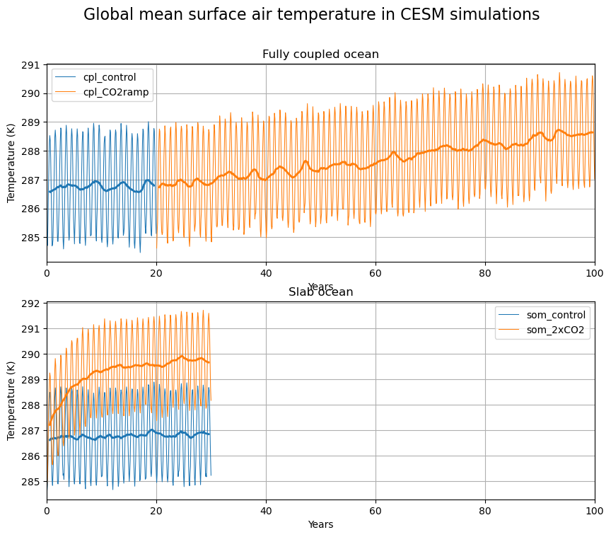
Let’s calculate the time series for global-, annual-mean near-surface air temperature.
print(atm['cpl_control'].TREFHT)

#  The area weighting needed for global averaging
gw = atm['som_control'].gw
print(gw)

def global_mean(field, weight=gw):
    '''Return the area-weighted global average of the input field'''
    return (field*weight).mean(dim=('lat','lon'))/weight.mean(dim='lat')

#  Loop through the four simulations and produce the global mean timeseries
TREFHT_global = {}
for name in casenames:
    TREFHT_global[name] = global_mean(atm[name].TREFHT)

fig, axes = plt.subplots(2,1,figsize=(10,8))
for name in casenames:
    if 'cpl' in name:
        ax = axes[0]
        ax.set_title('Fully coupled ocean')
    else:
        ax = axes[1]
        ax.set_title('Slab ocean')
    field = TREFHT_global[name]
    field_running = field.rolling(time=12, center=True).mean()
    line = ax.plot(field.time / days_per_year,
                   field,
                   label=name,
                   linewidth=0.75,
                   )
    ax.plot(field_running.time / days_per_year,
            field_running,
            color=line[0].get_color(),
            linewidth=2,
           )
for ax in axes:
    ax.legend();
    ax.set_xlabel('Years')
    ax.set_ylabel('Temperature (K)')
    ax.grid();
    ax.set_xlim(0,100)

fig.suptitle('Global mean surface air temperature in CESM simulations', fontsize=16);
<xarray.DataArray 'TREFHT' (time: 240, lat: 96, lon: 144)> Size: 13MB
[3317760 values with dtype=float32]
Coordinates:
  * time     (time) float64 2kB 31.0 59.0 90.0 ... 7.239e+03 7.269e+03 7.3e+03
  * lat      (lat) float64 768B -90.0 -88.11 -86.21 -84.32 ... 86.21 88.11 90.0
  * lon      (lon) float64 1kB 0.0 2.5 5.0 7.5 10.0 ... 350.0 352.5 355.0 357.5
Attributes:
    units:         K
    long_name:     Reference height temperature
    cell_methods:  time: mean
<xarray.DataArray 'gw' (lat: 96)> Size: 768B
[96 values with dtype=float64]
Coordinates:
  * lat      (lat) float64 768B -90.0 -88.11 -86.21 -84.32 ... 86.21 88.11 90.0
Attributes:
    long_name:  gauss weights
# extract the last 10 years from the slab ocean control simulation
# and the last 20 years from the coupled control
nyears_slab = 10
nyears_cpl = 20
clim_slice_slab = slice(-(nyears_slab*12),None)
clim_slice_cpl = slice(-(nyears_cpl*12),None)

# extract the last 10 years from the slab ocean control simulation
T0_slab = TREFHT_global['som_control'].isel(time=clim_slice_slab).mean(dim='time')
print(T0_slab)

# and the last 20 years from the coupled control
T0_cpl = TREFHT_global['cpl_control'].isel(time=clim_slice_cpl).mean(dim='time')
print(T0_cpl)

# extract the last 10 years from the slab 2xCO2 simulation
T2x_slab = TREFHT_global['som_2xCO2'].isel(time=clim_slice_slab).mean(dim='time')
print(T2x_slab)

# extract the last 20 years from the coupled CO2 ramp simulation
T2x_cpl = TREFHT_global['cpl_CO2ramp'].isel(time=clim_slice_cpl).mean(dim='time')
print(T2x_cpl)

ECS = T2x_slab - T0_slab
TCR = T2x_cpl - T0_cpl
print('The Equilibrium Climate Sensitivity is {:.3} K.'.format(float(ECS)))
print('The Transient Climate Response is {:.3} K.'.format(float(TCR)))
<xarray.DataArray ()> Size: 8B
array(286.82486457)
<xarray.DataArray ()> Size: 8B
array(286.75125938)
<xarray.DataArray ()> Size: 8B
array(289.71521445)
<xarray.DataArray ()> Size: 8B
array(288.41935278)
The Equilibrium Climate Sensitivity is 2.89 K.
The Transient Climate Response is 1.67 K.
Let’s check the spaital patterns:
# The map projection capabilities come from the cartopy package. There are many possible projections
import cartopy.crs as ccrs
from cartopy.util import add_cyclic_point
def make_map(field, title="", levels=8):
'''input field should be a 2D xarray.DataArray on a lat/lon grid.
Make a filled contour plot of the field, and a line plot of the zonal mean
'''
fig = plt.figure(figsize=(14,6))
nrows = 10; ncols = 3
mapax = plt.subplot2grid((nrows,ncols), (0,0), colspan=ncols-1, rowspan=nrows-1, projection=ccrs.Robinson())
barax = plt.subplot2grid((nrows,ncols), (nrows-1,0), colspan=ncols-1)
plotax = plt.subplot2grid((nrows,ncols), (0,ncols-1), rowspan=nrows-1)
# add cyclic point so cartopy doesn't show a white strip at zero longitude
wrap_data, wrap_lon = add_cyclic_point(field.values, coord=field.lon, axis=field.dims.index('lon'))
cx = mapax.contourf(wrap_lon, field.lat, wrap_data, levels=levels, transform=ccrs.PlateCarree())
mapax.set_global(); mapax.coastlines();
plt.colorbar(cx, cax=barax, orientation='horizontal', label='Surface air temperature (K)')
plotax.plot(field.mean(dim='lon'), field.lat)
plotax.set_xlabel('Zonal mean (K)')
plotax.set_ylabel('Latitude')
plotax.grid()
fig.suptitle(title, fontsize=16)
return fig, (mapax, plotax, barax), cx
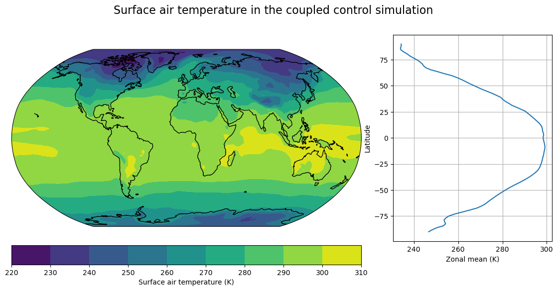
# Plot a single time slice of surface air temperature just as example
fig, axes, cx = make_map(atm['cpl_control'].TREFHT.isel(time=0),
title="Surface air temperature in the coupled control simulation")
Tmap_cpl_2x = atm['cpl_CO2ramp'].TREFHT.isel(time=clim_slice_cpl).mean(dim='time')
Tmap_cpl_control = atm['cpl_control'].TREFHT.isel(time=clim_slice_cpl).mean(dim='time')
DeltaT_cpl = Tmap_cpl_2x - Tmap_cpl_control
Tmap_som_2x = atm['som_2xCO2'].TREFHT.isel(time=clim_slice_slab).mean(dim='time')
Tmap_som_control = atm['som_control'].TREFHT.isel(time=clim_slice_slab).mean(dim='time')
DeltaT_som = Tmap_som_2x - Tmap_som_control
contours = np.arange(0., 8.5, 0.5)
fig, axes, cx = make_map(DeltaT_cpl, levels=contours,
title="Surface air temperature anomaly (coupled transient)")
axes[1].set_xlim(0,7) # ensure the line plots have same axes
fig, axes,cx = make_map(DeltaT_som, levels=contours,
title="Surface air temperature anomaly (equilibrium SOM)")
axes[1].set_xlim(0,7)
(0.0, 7.0)
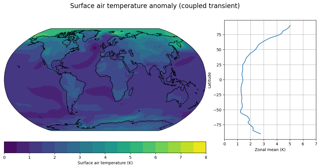
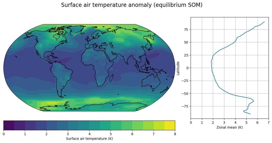
Polar amplification
Land-sea contrast
North Atlantic warming hole
Delayed warming of the Southern Ocean
Transient response in simple models#
%matplotlib inline
import numpy as np
import matplotlib.pyplot as plt
import xarray as xr
import climlab

# Get the water vapor data from CESM output
cesm_data_path = "~/Desktop/ebooks/data/"
atm_control = xr.open_dataset(cesm_data_path + "cpl_1850_f19.cam.h0.nc")
# Take global, annual average of the specific humidity
weight_factor = atm_control.gw / atm_control.gw.mean(dim='lat')
Qglobal = (atm_control.Q * weight_factor).mean(dim=('lat','lon','time'))

#  Make a model on same vertical domain as the GCM
state = climlab.column_state(lev=Qglobal.lev, water_depth=2.5)
steps_per_year = 90
deltat = climlab.constants.seconds_per_year/steps_per_year
rad = climlab.radiation.RRTMG(name='Radiation',
                              state=state,
                              specific_humidity=Qglobal.values,
                              timestep = deltat,
                              albedo = 0.25,  # tuned to give reasonable ASR for reference cloud-free model
                             )
conv = climlab.convection.ConvectiveAdjustment(name='Convection',
                                               state=state,
                                               adj_lapse_rate=6.5,
                                               timestep=rad.timestep,)
rcm_control = climlab.couple([rad,conv], name='Radiative-Convective Model')

rcm_control.integrate_years(5)
rcm_control.ASR - rcm_control.OLR

slab_control = []
slab_control.append(rcm_control)
slab_control.append(climlab.process_like(rcm_control))

slab_2x = []
for n in range(len(slab_control)):
    rcm_2xCO2 = climlab.process_like(rcm_control)
    rcm_2xCO2.subprocess['Radiation'].absorber_vmr['CO2'] *= 2.
    if n == 0:
        rcm_2xCO2.name = 'High-sensitivity RCM'
    elif n == 1:
        rcm_2xCO2.name = 'Low-sensitivity RCM'
    slab_2x.append(rcm_2xCO2)

#  actual specific humidity
q = rcm_control.subprocess['Radiation'].specific_humidity
#  saturation specific humidity (a function of temperature and pressure)
qsat = climlab.utils.thermo.qsat(rcm_control.Tatm, rcm_control.lev)
#  Relative humidity (stay fixed!)
rh = q/qsat
Integrating for 450 steps, 1826.2110000000002 days, or 5 years.
Total elapsed time is 5.000000000000044 years.
We change lapse rate:
lapse_change_factor = [+0.3, -0.3]

for n in range(len(slab_2x)):
    rcm_2xCO2 = slab_2x[n]
    print('Integrating ' + rcm_2xCO2.name)
    for m in range(5 * steps_per_year):
        # At every timestep
        # we calculate the new saturation specific humidity for the new temperature
        #  and change the water vapor in the radiation model
        #  so that relative humidity is always the same
        qsat = climlab.utils.thermo.qsat(rcm_2xCO2.Tatm, rcm_2xCO2.lev)
        rcm_2xCO2.subprocess['Radiation'].specific_humidity[:] = rh * qsat
        #  We also adjust the critical lapse rate in our convection model
        DeltaTs = rcm_2xCO2.Ts - rcm_control.Ts
        rcm_2xCO2.subprocess['Convection'].adj_lapse_rate = 6.5 + lapse_change_factor[n]*DeltaTs
        rcm_2xCO2.step_forward()
    imbalance = (rcm_2xCO2.ASR - rcm_2xCO2.OLR).squeeze()  # convert to a single scalar
    ecs = (rcm_2xCO2.Ts - rcm_control.Ts).squeeze()
    print('The TOA imbalance is {:.2e} W/m2'.format(imbalance))
    print('The ECS is {:.2f} K'.format(ecs))
    print('')
Integrating High-sensitivity RCM
The TOA imbalance is 3.11e-05 W/m2
The ECS is 3.57 K

Integrating Low-sensitivity RCM
The TOA imbalance is 2.22e-04 W/m2
The ECS is 2.22 K
Why the lapse rates affect the climate sensitivity?
The current models have too shallow water depth, which means small heat capacity and reaching equilibrium very fast.
print(slab_control[0].depth_bounds)
[0. 2.5]
We need deeper ocean for ocean heat uptake.
#  Create the domains
ocean_bounds = np.arange(0., 2010., 100.)
depthax = climlab.Axis(axis_type='depth', bounds=ocean_bounds)
ocean = climlab.domain.domain.Ocean(axes=depthax)
atm = slab_control[0].Tatm.domain

#  Model 0 has a higher ocean heat diffusion coefficient --
#  a more efficent deep ocean heat sink
ocean_diff = [5.E-4, 3.5E-4]

#  List of deep ocean models
deep = []
for n in range(len(slab_control)):
    rcm_control = slab_control[n]
    #  Create the state variables
    Tinitial_ocean = rcm_control.Ts * np.ones(ocean.shape)
    Tocean = climlab.Field(Tinitial_ocean.copy(), domain=ocean)
    Tatm = climlab.Field(rcm_control.Tatm.copy(), domain=atm)

    #  Surface temperature Ts is the upper-most grid box of the ocean
    Ts = Tocean[0:1]
    atm_state = {'Tatm': Tatm, 'Ts': Ts}

    rad = climlab.radiation.RRTMG(name='Radiation',
                                  state=atm_state,
                                  specific_humidity=Qglobal.values,
                                  timestep = deltat,
                                  albedo = 0.25,
                                 )
    conv = climlab.convection.ConvectiveAdjustment(name='Convection',
                                                   state=atm_state,
                                                   adj_lapse_rate=6.5,
                                                   timestep=rad.timestep,)

    model = rad + conv
    if n == 0:
        model.name = 'RCM with high sensitivity and efficient heat uptake'
    elif n == 1:
        model.name = 'RCM with low sensitivity and inefficient heat uptake'
    model.set_state('Tocean', Tocean)
    diff = climlab.dynamics.Diffusion(state={'Tocean': model.Tocean},
                                K=ocean_diff[n],
                                diffusion_axis='depth',
                                timestep=deltat * 10,)
    model.add_subprocess('Ocean Heat Uptake', diff)
    print('')
    print(model)
    print('')
    deep.append(model)
climlab Process of type <class 'climlab.process.time_dependent_process.TimeDependentProcess'>.
State variables and domain shapes:
  Tatm: (26,)
  Ts: (1,)
  Tocean: (20,)
The subprocess tree:
RCM with high sensitivity and efficient heat uptake: <class 'climlab.process.time_dependent_process.TimeDependentProcess'>
   Radiation: <class 'climlab.radiation.rrtm.rrtmg.RRTMG'>
      SW: <class 'climlab.radiation.rrtm.rrtmg_sw.RRTMG_SW'>
      LW: <class 'climlab.radiation.rrtm.rrtmg_lw.RRTMG_LW'>
   Convection: <class 'climlab.convection.convadj.ConvectiveAdjustment'>
   Ocean Heat Uptake: <class 'climlab.dynamics.advection_diffusion.Diffusion'>


climlab Process of type <class 'climlab.process.time_dependent_process.TimeDependentProcess'>.
State variables and domain shapes:
  Tatm: (26,)
  Ts: (1,)
  Tocean: (20,)
The subprocess tree:
RCM with low sensitivity and inefficient heat uptake: <class 'climlab.process.time_dependent_process.TimeDependentProcess'>
   Radiation: <class 'climlab.radiation.rrtm.rrtmg.RRTMG'>
      SW: <class 'climlab.radiation.rrtm.rrtmg_sw.RRTMG_SW'>
      LW: <class 'climlab.radiation.rrtm.rrtmg_lw.RRTMG_LW'>
   Convection: <class 'climlab.convection.convadj.ConvectiveAdjustment'>
   Ocean Heat Uptake: <class 'climlab.dynamics.advection_diffusion.Diffusion'>
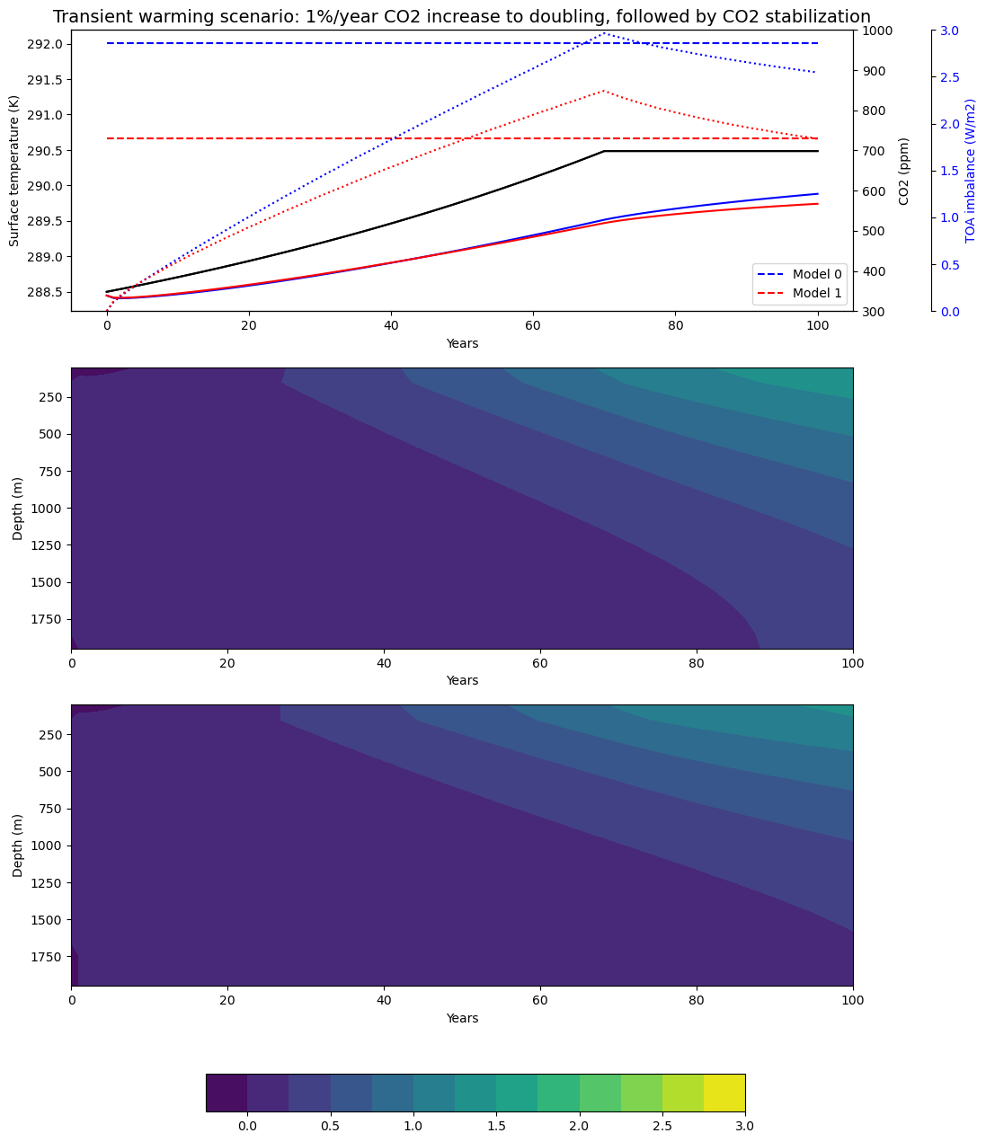
We now increase CO2 by 1% per year to doucling its concentration, which takes about 70 years.
num_years = 100
years = np.arange(num_years+1)

Tsarray = []
Tocean = []
netrad = []
for n in range(len(deep)):
    thisTs = np.nan * np.zeros(num_years+1)
    thisnetrad = np.nan * np.zeros(num_years+1)
    thisTocean = np.nan * np.zeros((deep[n].Tocean.size, num_years+1))
    thisTs[0] = deep[n].Ts.squeeze()
    thisnetrad[0] = (deep[n].ASR - deep[n].OLR).squeeze()
    thisTocean[:, 0] = deep[n].Tocean
    Tsarray.append(thisTs)
    Tocean.append(thisTocean)
    netrad.append(thisnetrad)

CO2initial = deep[0].subprocess['Radiation'].absorber_vmr['CO2']
CO2array = np.nan * np.zeros(num_years+1)
CO2array[0] = CO2initial * 1E6

#  Increase CO2 by 1% / year for 70 years (until doubled), and then hold constant
for y in range(num_years):
    if deep[0].subprocess['Radiation'].absorber_vmr['CO2'] < 2 * CO2initial:
        for model in deep:
            model.subprocess['Radiation'].absorber_vmr['CO2'] *= 1.01
    CO2array[y+1] = deep[0].subprocess['Radiation'].absorber_vmr['CO2'] * 1E6
    if np.mod(y,10) == 0:
       print('Year ', y+1, ', CO2 mixing ratio is ', CO2array[y+1],' ppm.')

    for n, model in enumerate(deep):
        for m in range(steps_per_year):
            qsat = climlab.utils.thermo.qsat(model.Tatm, model.lev)
            model.subprocess['Radiation'].specific_humidity[:] = rh * qsat
            DeltaTs = model.Ts - slab_control[n].Ts
            model.subprocess['Convection'].adj_lapse_rate = 6.5 + lapse_change_factor[n]*DeltaTs
            model.step_forward()

            Tsarray[n][y+1] = model.Ts.squeeze()
            Tocean[n][:, y+1] = model.Tocean
            netrad[n][y+1] = (model.ASR - model.OLR).squeeze()
Year 1 , CO2 mixing ratio is 351.47999999999996 ppm.
Year 11 , CO2 mixing ratio is 388.2525846395302 ppm.
Year 21 , CO2 mixing ratio is 428.87239524091143 ppm.
Year 31 , CO2 mixing ratio is 473.7419367612098 ppm.
Year 41 , CO2 mixing ratio is 523.3058250815881 ppm.
Year 51 , CO2 mixing ratio is 578.0551927416877 ppm.
Year 61 , CO2 mixing ratio is 638.5325556113066 ppm.
Year 71 , CO2 mixing ratio is 698.3536522015938 ppm.
Year 81 , CO2 mixing ratio is 698.3536522015938 ppm.
Year 91 , CO2 mixing ratio is 698.3536522015938 ppm.
colorlist = ['b', 'r']
co2color = 'k'

num_axes = len(deep) + 1
fig, ax = plt.subplots(num_axes, figsize=(12,14))

# Twin the x-axis twice to make independent y-axes.
topaxes = [ax[0], ax[0].twinx(), ax[0].twinx()]

# Make some space on the right side for the extra y-axis.
fig.subplots_adjust(right=0.85)

# Move the last y-axis spine over to the right by 10% of the width of the axes
topaxes[-1].spines['right'].set_position(('axes', 1.1))

# To make the border of the right-most axis visible, we need to turn the frame
# on. This hides the other plots, however, so we need to turn its fill off.
topaxes[-1].set_frame_on(True)
topaxes[-1].patch.set_visible(False)

for n, model in enumerate(slab_2x):
    topaxes[0].plot(model.Ts*np.ones_like(Tsarray[n]), '--', color=colorlist[n])
topaxes[0].set_ylabel('Surface temperature (K)')
topaxes[0].set_xlabel('Years')
topaxes[0].set_title('Transient warming scenario: 1%/year CO2 increase to doubling, followed by CO2 stabilization', fontsize=14)
topaxes[0].legend(['Model 0', 'Model 1'], loc='lower right')

topaxes[1].plot(CO2array, color=co2color)
topaxes[1].set_ylabel('CO2 (ppm)', color=co2color)
for tl in topaxes[1].get_yticklabels():
    tl.set_color(co2color)
topaxes[1].set_ylim(300., 1000.)

topaxes[2].set_ylabel('TOA imbalance (W/m2)', color='b')
for tl in topaxes[2].get_yticklabels():
    tl.set_color('b')
topaxes[2].set_ylim(0, 3)


contour_levels = np.arange(-0.25, 3.25, 0.25)
for n in range(len(deep)):
    cax = ax[n+1].contourf(years, deep[n].depth, Tocean[n] - Tsarray[n][0], levels=contour_levels)
    ax[n+1].invert_yaxis()
    ax[n+1].set_ylabel('Depth (m)')
    ax[n+1].set_xlabel('Years')


for n, model in enumerate(deep):
    topaxes[0].plot(Tsarray[n], color=colorlist[n])
    topaxes[2].plot(netrad[n], ':', color=colorlist[n])
    for n in range(len(deep)):
        cax = ax[n+1].contourf(years, deep[n].depth, Tocean[n] - Tsarray[n][0], levels=contour_levels)
topaxes[1].plot(CO2array, color=co2color)

fig.subplots_adjust(bottom=0.12)
cbar_ax = fig.add_axes([0.25, 0.02, 0.5, 0.03])
fig.colorbar(cax, cax=cbar_ax, orientation='horizontal');
Homework assignment X (due xxx)#
Please change adj_lapse_rate = 9.8. This is the dry adiabatic lapse rate. Calculate the water feedback parameter in this scenario.