16. Ice Albedo Feedback in EBM#
Note
The Python scripts used below and some materials are modified from Prof. Brian E. J. Rose’s climlab website.
Interactive ice/snow line (step function)#
The idea is to change the albedo as a function of latitude and a threshold temperatre \(T_{f} = -10 ^{o}C\). This is historically inheritated from Budyko’s model.
where \(P_{2}(sin(\phi))=\frac{1}{2}(3\sin(\phi)^{2}-1)\).
%matplotlib inline
import numpy as np
import matplotlib.pyplot as plt
import climlab
from climlab import constants as const
# for convenience, set up a dictionary with our reference parameters
param = {'D':0.55, 'A':210, 'B':2, 'a0':0.3, 'a2':0.078, 'ai':0.62, 'Tf':-10.}
model1 = climlab.EBM_annual(name='EBM with interactive ice line',
num_lat=180,
D=0.55,
A=210.,
B=2.,
Tf=-10.,
a0=0.3,
a2=0.078,
ai=0.62)
print(model1)
print(model1.param)
# A python shortcut... we can use the dictionary to pass lots of input arguments simultaneously:
# same thing as before, but written differently:
model1 = climlab.EBM_annual(name='EBM with interactive ice line',
num_lat=180,
**param)
print(model1)
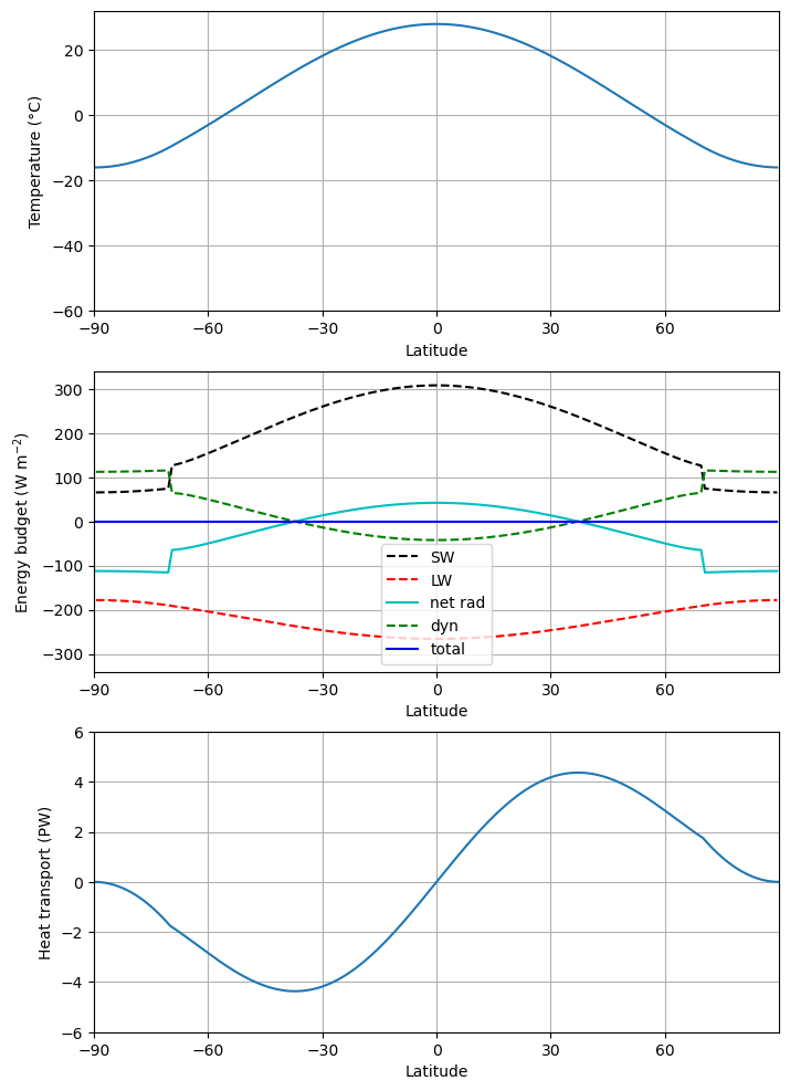
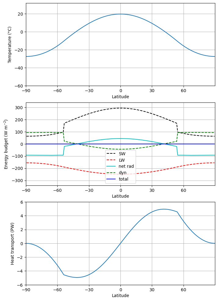
def ebm_plot(e, return_fig=False):
templimits = -60,32
radlimits = -340, 340
htlimits = -6,6
latlimits = -90,90
lat_ticks = np.arange(-90,90,30)
fig = plt.figure(figsize=(8,12))
ax1 = fig.add_subplot(3,1,1)
ax1.plot(e.lat, e.Ts)
ax1.set_ylim(templimits)
ax1.set_ylabel('Temperature (°C)')
ax2 = fig.add_subplot(3,1,2)
ax2.plot(e.lat, e.ASR, 'k--', label='SW' )
ax2.plot(e.lat, -e.OLR, 'r--', label='LW' )
ax2.plot(e.lat, e.net_radiation, 'c-', label='net rad' )
ax2.plot(e.lat, e.heat_transport_convergence, 'g--', label='dyn' )
ax2.plot(e.lat, e.net_radiation + e.heat_transport_convergence, 'b-', label='total' )
ax2.set_ylim(radlimits)
ax2.set_ylabel('Energy budget (W m$^{-2}$)')
ax2.legend()
ax3 = fig.add_subplot(3,1,3)
ax3.plot(e.lat_bounds, e.heat_transport )
ax3.set_ylim(htlimits)
ax3.set_ylabel('Heat transport (PW)')
for ax in [ax1, ax2, ax3]:
ax.set_xlabel('Latitude')
ax.set_xlim(latlimits)
ax.set_xticks(lat_ticks)
ax.grid()
if return_fig:
return fig
model1.integrate_years(5)
model1.ASR.to_xarray()
climlab.global_mean(model1.ASR - model1.OLR)
# Integrate out to equilibrium.
model1.integrate_years(5)
# Check for energy balance
print(climlab.global_mean(model1.net_radiation))
f = ebm_plot(model1)
# There is a diagnostic that tells us the current location of the ice edge:
model1.icelat
climlab Process of type <class 'climlab.model.ebm.EBM_annual'>.
State variables and domain shapes:
  Ts: (180, 1)
The subprocess tree:
EBM with interactive ice line: <class 'climlab.model.ebm.EBM_annual'>
   LW: <class 'climlab.radiation.aplusbt.AplusBT'>
   insolation: <class 'climlab.radiation.insolation.AnnualMeanInsolation'>
   albedo: <class 'climlab.surface.albedo.StepFunctionAlbedo'>
      iceline: <class 'climlab.surface.albedo.Iceline'>
      warm_albedo: <class 'climlab.surface.albedo.P2Albedo'>
      cold_albedo: <class 'climlab.surface.albedo.ConstantAlbedo'>
   SW: <class 'climlab.radiation.absorbed_shorwave.SimpleAbsorbedShortwave'>
   diffusion: <class 'climlab.dynamics.meridional_heat_diffusion.MeridionalHeatDiffusion'>

{'timestep': 350632.51200000005, 'S0': 1365.2, 's2': -0.48, 'A': 210.0, 'B': 2.0, 'D': 0.55, 'Tf': -10.0, 'water_depth': 10.0, 'a0': 0.3, 'a2': 0.078, 'ai': 0.62}
climlab Process of type <class 'climlab.model.ebm.EBM_annual'>.
State variables and domain shapes:
  Ts: (180, 1)
The subprocess tree:
EBM with interactive ice line: <class 'climlab.model.ebm.EBM_annual'>
   LW: <class 'climlab.radiation.aplusbt.AplusBT'>
   insolation: <class 'climlab.radiation.insolation.AnnualMeanInsolation'>
   albedo: <class 'climlab.surface.albedo.StepFunctionAlbedo'>
      iceline: <class 'climlab.surface.albedo.Iceline'>
      warm_albedo: <class 'climlab.surface.albedo.P2Albedo'>
      cold_albedo: <class 'climlab.surface.albedo.ConstantAlbedo'>
   SW: <class 'climlab.radiation.absorbed_shorwave.SimpleAbsorbedShortwave'>
   diffusion: <class 'climlab.dynamics.meridional_heat_diffusion.MeridionalHeatDiffusion'>

Integrating for 450 steps, 1826.2110000000002 days, or 5 years.
Total elapsed time is 5.000000000000044 years.
Integrating for 450 steps, 1826.2110000000002 days, or 5 years.
Total elapsed time is 9.999999999999863 years.
1.2815863495813735e-05
array([-70., 70.])
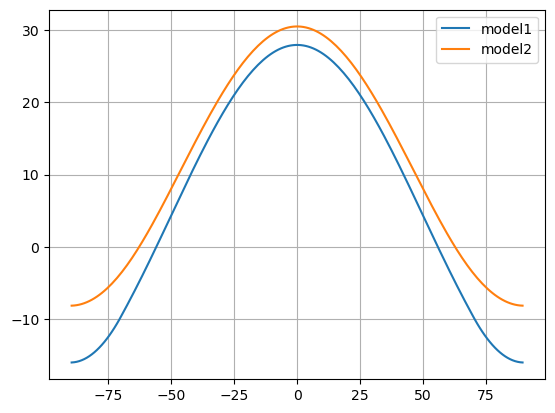
Polar-amplified warming in EBM (Yeah!!!)#
If we consider a scenario of doubling CO2, that is to change paraemter \(A\) to \(A-\delta A\), where \(\delta A= 4\) W/m\(^2\).
model1.subprocess['LW'].A

deltaA = 4.

#  This is a very handy way to "clone" an existing model:
model2 = climlab.process_like(model1)

#  Now change the longwave parameter:
model2.subprocess['LW'].A = param['A'] - deltaA
#  and integrate out to equilibrium again
model2.integrate_years(5, verbose=False)

plt.plot(model1.lat, model1.Ts, label='model1')
plt.plot(model2.lat, model2.Ts, label='model2')
plt.legend(); plt.grid()

model2.icelat
array([-90., 90.])
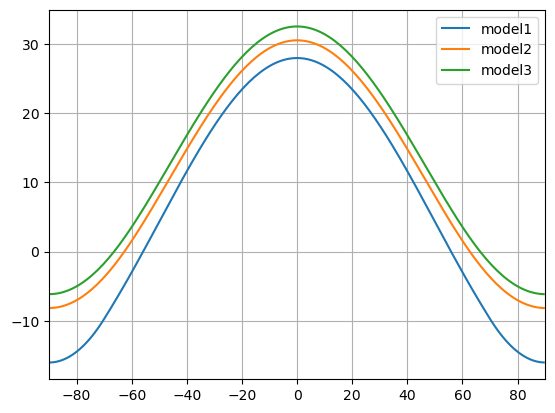
model3 = climlab.process_like(model1)
model3.subprocess['LW'].A = param['A'] - 2*deltaA
model3.integrate_years(5, verbose=False)

plt.plot(model1.lat, model1.Ts, label='model1')
plt.plot(model2.lat, model2.Ts, label='model2')
plt.plot(model3.lat, model3.Ts, label='model3')
plt.xlim(-90, 90)
plt.grid()
plt.legend()
<matplotlib.legend.Legend at 0x143713910>
For me, this is the minimal model to produce polar amplification. Starting from this model, I want to increase the model hierachy to study the drivers of polar mechanism.
Solar forcing#
m = climlab.EBM_annual(num_lat=180, **param)
#  The current (default) solar constant, corresponding to present-day conditions:
m.subprocess.insolation.S0

#  First, get to equilibrium
m.integrate_years(5.)
#  Check for energy balance
climlab.global_mean(m.net_radiation)

m.icelat

#  Now make the solar constant smaller:
m.subprocess.insolation.S0 = 1300.

#  Integrate to new equilibrium
m.integrate_years(10.)
#  Check for energy balance
climlab.global_mean(m.net_radiation)

m.icelat

ebm_plot(m)
Integrating for 450 steps, 1826.2110000000002 days, or 5.0 years.
Total elapsed time is 5.000000000000044 years.
Integrating for 900 steps, 3652.4220000000005 days, or 10.0 years.
Total elapsed time is 14.999999999999647 years.
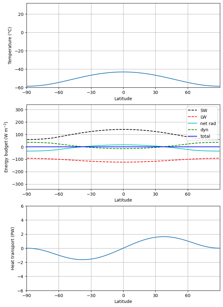
Ice cap instability#
If we continue decreasing solar insolation:
#  Now make the solar constant smaller:
m.subprocess.insolation.S0 = 1200.
#  First, get to equilibrium
m.integrate_years(5.)
#  Check for energy balance
climlab.global_mean(m.net_radiation)

m.integrate_years(10.)
#  Check for energy balance
climlab.global_mean(m.net_radiation)

ebm_plot(m)

m.icelat
Integrating for 450 steps, 1826.2110000000002 days, or 5.0 years.
Total elapsed time is 19.99999999999943 years.
Integrating for 900 steps, 3652.4220000000005 days, or 10.0 years.
Total elapsed time is 30.000000000000693 years.
array([-0., 0.])
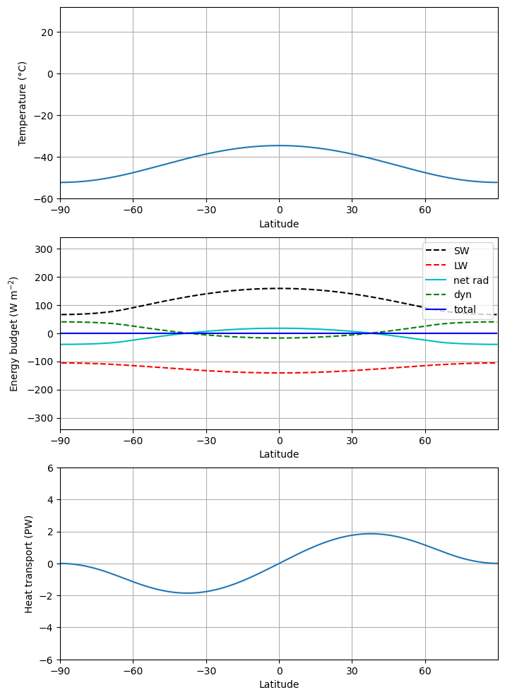
If we now trun it back to present-day value:
#  Now make the solar constant smaller:
m.subprocess.insolation.S0 = 1365.2
#  First, get to equilibrium
m.integrate_years(5.)
#  Check for energy balance
climlab.global_mean(m.net_radiation)

ebm_plot(m)
Integrating for 450 steps, 1826.2110000000002 days, or 5.0 years.
Total elapsed time is 35.0000000000016 years.
Homework assignment X (due xxx)#
Solar forcing. Please change the solar forcing and discuss the results.
m = climlab.EBM_annual(num_lat=180, **param)
#  The current (default) solar constant, corresponding to present-day conditions:
m.subprocess.insolation.S0

#  First, get to equilibrium
m.integrate_years(5.)
#  Check for energy balance
climlab.global_mean(m.net_radiation)

m.icelat

#  Now make the solar constant smaller:
m.subprocess.insolation.S0 = 1300.

#  Integrate to new equilibrium
m.integrate_years(10.)
#  Check for energy balance
climlab.global_mean(m.net_radiation)

m.icelat

ebm_plot(m)
Integrating for 450 steps, 1826.2110000000002 days, or 5.0 years.
Total elapsed time is 5.000000000000044 years.
Integrating for 900 steps, 3652.4220000000005 days, or 10.0 years.
Total elapsed time is 14.999999999999647 years.