18. Snowball Earth#
Note
The Python scripts used below and some materials are modified from Prof. Brian E. J. Rose’s climlab website.
The snowball Earth hypothesis#
Various bizarre features in the geological record from 635 and 715 Ma ago indicate that the Earth underwent some very extreme environmental changes at least twice. The Snowball Earth hypothesis postulates that:
The Earth was completely ice-covered (including the oceans)
The total glaciation endured for millions of years
CO2 slowly accumulated in the atmosphere from volcanoes
Weathering of rocks (normally acting to reduce CO2) extremely slow due to cold, dry climate
Eventually the extreme greenhouse effect is enough to melt back the ice
The Earth then enters a period of extremely hot climate.
The hypothesis rests on a phenomenon first discovered by climate modelers in the Budyko-Sellers EBM: runaway ice-albedo feedback or large ice cap instability.
Large ice cap instability#
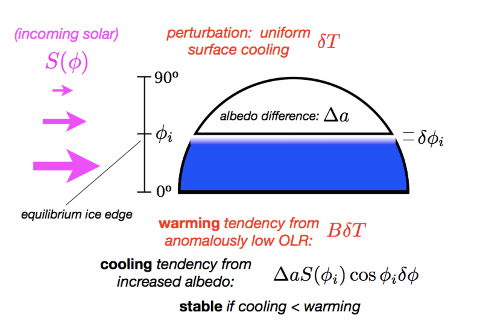
Fig. 55 Fiture credit to: Professor Brian E. J. Rose#
The displancement of ice edge is \(\delta \phi\), so the cooling tendency due to albedo change is:
The warming tendency due to outgoing lownwave reduction is:
If warming tendency is larger than cooling tendency, then the system can reach an equilibrium state.
If not, what will happen? \(\frac{\delta \alpha S(\phi_{i})\cos(\phi_{i})}{B}\) is large in low latitudes, so the ice grows toward the south before it reaches an equilibrium state.
Note
You may need to run this script on your workstation.
%matplotlib inline
import numpy as np
import matplotlib.pyplot as plt
from climlab import constants as const
import climlab
# for convenience, set up a dictionary with our reference parameters
param = {'A':210, 'B':2, 'a0':0.3, 'a2':0.078, 'ai':0.62, 'Tf':-10., 'D':0.55}
model1 = climlab.EBM_annual(name='Annual Mean EBM with ice line', num_lat=90, **param )
print(model1)
model1.integrate_years(5)
Tequil = np.array(model1.Ts)
ALBequil = np.array(model1.albedo)
OLRequil = np.array(model1.OLR)
ASRequil = np.array(model1.ASR)
model1.Ts -= 20.
model1.compute_diagnostics()
my_ticks = [-90,-60,-30,0,30,60,90]
lat = model1.lat
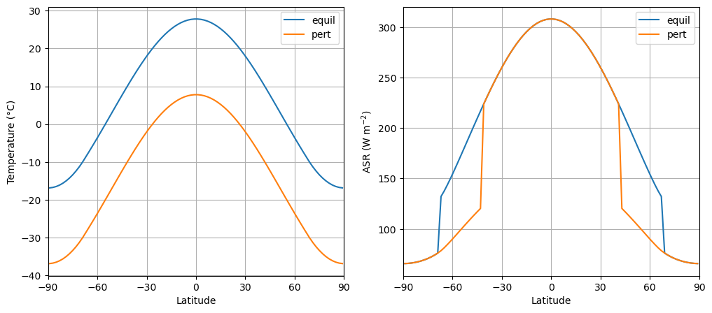
fig = plt.figure( figsize=(12,5) )
ax1 = fig.add_subplot(1,2,1)
ax1.plot(lat, Tequil, label='equil')
ax1.plot(lat, model1.state['Ts'], label='pert' )
ax1.grid()
ax1.legend()
ax1.set_xlim(-90,90)
ax1.set_xticks(my_ticks)
ax1.set_xlabel('Latitude')
ax1.set_ylabel('Temperature (°C)')
ax2 = fig.add_subplot(1,2,2)
ax2.plot( lat, ASRequil, label='equil')
ax2.plot( lat, model1.diagnostics['ASR'], label='pert' )
ax2.grid()
ax2.legend()
ax2.set_xlim(-90,90)
ax2.set_xticks(my_ticks)
ax2.set_xlabel('Latitude')
ax2.set_ylabel('ASR (W m$^{-2}$)')
print(climlab.global_mean( model1.ASR - ASRequil ))
climlab Process of type <class 'climlab.model.ebm.EBM_annual'>.
State variables and domain shapes:
  Ts: (90, 1)
The subprocess tree:
Annual Mean EBM with ice line: <class 'climlab.model.ebm.EBM_annual'>
   LW: <class 'climlab.radiation.aplusbt.AplusBT'>
   insolation: <class 'climlab.radiation.insolation.AnnualMeanInsolation'>
   albedo: <class 'climlab.surface.albedo.StepFunctionAlbedo'>
      iceline: <class 'climlab.surface.albedo.Iceline'>
      warm_albedo: <class 'climlab.surface.albedo.P2Albedo'>
      cold_albedo: <class 'climlab.surface.albedo.ConstantAlbedo'>
   SW: <class 'climlab.radiation.absorbed_shorwave.SimpleAbsorbedShortwave'>
   diffusion: <class 'climlab.dynamics.meridional_heat_diffusion.MeridionalHeatDiffusion'>

Integrating for 450 steps, 1826.2110000000002 days, or 5 years.
Total elapsed time is 5.000000000000044 years.
-19.726674194909386
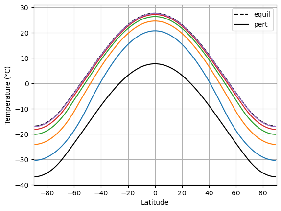
We can calculate the feedback parameter:
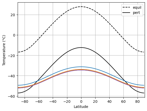
plt.plot( lat, Tequil, 'k--', label='equil' )
plt.plot( lat, model1.Ts, 'k-', label='pert' )
plt.grid(); plt.xlim(-90,90); plt.legend()
for n in range(5):
    model1.integrate_years(years=1.0, verbose=False)
    plt.plot(lat, model1.Ts)
plt.ylabel('Temperature (°C)')
plt.xlabel('Latitude')
Text(0.5, 0, 'Latitude')
model1.Ts -= 40.
model1.compute_diagnostics()

print(climlab.global_mean( model1.ASR - ASRequil ))

plt.plot( lat, Tequil, 'k--', label='equil' )
plt.plot( lat, model1.Ts, 'k-', label='pert' )
plt.grid(); plt.xlim(-90,90); plt.legend()
for n in range(5):
    model1.integrate_years(years=1.0, verbose=False)
    plt.plot(lat, model1.Ts)
plt.ylabel('Temperature (°C)')
plt.xlabel('Latitude')
-108.34822044773354
Text(0.5, 0, 'Latitude')
We again calculate the feedback parameter:
Below the code may not be run on your laptop.
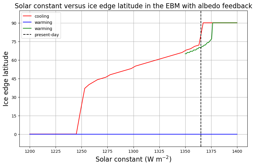
Hysteresis#
model2 = climlab.EBM_annual(num_lat = 180, **param)
S0array = np.linspace(1400., 1200., 50)
model2.integrate_years(5)

print( model2.icelat)

icelat_cooling = np.empty_like(S0array)
icelat_warming = np.empty_like(S0array)

# First cool....
for n in range(S0array.size):
    model2.subprocess['insolation'].S0 = S0array[n]
    model2.integrate_years(10, verbose=False)
    icelat_cooling[n] = np.max(model2.icelat)
Integrating for 450 steps, 1826.2110000000002 days, or 5 years.
Total elapsed time is 5.000000000000044 years.
[-70.  70.]
# Then warm...
for n in range(S0array.size):
    model2.subprocess['insolation'].S0 = np.flipud(S0array)[n]
    model2.integrate_years(10, verbose=False)
    icelat_warming[n] = np.max(model2.icelat)
model3 = climlab.EBM_annual(num_lat=180, **param)
S0array3 = np.linspace(1350., 1400., 50)
#S0array3 = np.linspace(1350., 1400., 5)
icelat3 = np.empty_like(S0array3)
for n in range(S0array3.size):
    model3.subprocess['insolation'].S0 = S0array3[n]
    model3.integrate_years(10, verbose=False)
    icelat3[n] = np.max(model3.icelat)

fig = plt.figure( figsize=(10,6) )
ax = fig.add_subplot(111)
ax.plot(S0array, icelat_cooling, 'r-', label='cooling' )
ax.plot(S0array, icelat_warming, 'b-', label='warming' )
ax.plot(S0array3, icelat3, 'g-', label='warming' )
ax.set_ylim(-10,100)
ax.set_yticks((0,15,30,45,60,75,90))
ax.grid()
ax.set_ylabel('Ice edge latitude', fontsize=16)
ax.set_xlabel('Solar constant (W m$^{-2}$)', fontsize=16)
ax.plot( [const.S0, const.S0], [-10, 100], 'k--', label='present-day' )
ax.legend(loc='upper left')
ax.set_title('Solar constant versus ice edge latitude in the EBM with albedo feedback', fontsize=16);
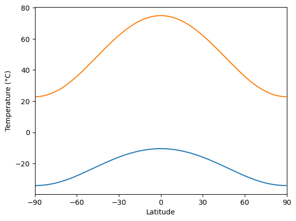
model4 = climlab.process_like(model2)  # initialize with cold Snowball temperature
model4.subprocess['insolation'].S0 = 1830.
model4.integrate_years(40)
plt.plot(model4.lat, model4.Ts)
plt.xlim(-90,90); plt.ylabel('Temperature (°C)'); plt.xlabel('Latitude')
plt.grid(); plt.xticks(my_ticks)
print('The ice edge is at ' + str(model4.icelat) + ' degrees latitude.' )

model4.subprocess['insolation'].S0 = 1840.
model4.integrate_years(10)
plt.plot(model4.lat, model4.Ts)
plt.xlim(-90,90); plt.ylabel('Temperature (°C)'); plt.xlabel('Latitude')
plt.grid(); plt.xticks(my_ticks);

print( model4.global_mean_temperature() )
Integrating for 3600 steps, 14609.688000000002 days, or 40 years.
Total elapsed time is 1045.000000000071 years.
The ice edge is at [-0.  0.] degrees latitude.
Integrating for 900 steps, 3652.4220000000005 days, or 10 years.
Total elapsed time is 1055.0000000001087 years.
57.73267527507378
S0array_snowballmelt = np.linspace(1400., 1900., 50)
icelat_snowballmelt = np.empty_like(S0array_snowballmelt)
icelat_snowballmelt_cooling = np.empty_like(S0array_snowballmelt)

for n in range(S0array_snowballmelt.size):
    model2.subprocess['insolation'].S0 = S0array_snowballmelt[n]
    model2.integrate_years(10, verbose=False)
    icelat_snowballmelt[n] = np.max(model2.icelat)
for n in range(S0array_snowballmelt.size):
    model2.subprocess['insolation'].S0 = np.flipud(S0array_snowballmelt)[n]
    model2.integrate_years(10, verbose=False)
    icelat_snowballmelt_cooling[n] = np.max(model2.icelat)


fig = plt.figure( figsize=(10,6) )
ax = fig.add_subplot(111)
ax.plot(S0array, icelat_cooling, 'r-', label='cooling' )
ax.plot(S0array, icelat_warming, 'b-', label='warming' )
ax.plot(S0array3, icelat3, 'g-', label='warming' )
ax.plot(S0array_snowballmelt, icelat_snowballmelt, 'b-' )
ax.plot(S0array_snowballmelt, icelat_snowballmelt_cooling, 'r-' )
ax.set_ylim(-10,100)
ax.set_yticks((0,15,30,45,60,75,90))
ax.grid()
ax.set_ylabel('Ice edge latitude', fontsize=16)
ax.set_xlabel('Solar constant (W m$^{-2}$)', fontsize=16)
ax.plot( [const.S0, const.S0], [-10, 100], 'k--', label='present-day' )
ax.legend(loc='upper left')
ax.set_title('Solar constant versus ice edge latitude in the EBM with albedo feedback', fontsize=16);
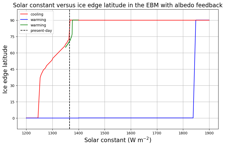
From the above results, we can conclude:
For extremely large \(S_0\), the only possible climate is a hot Earth with no ice.
For extremely small \(S_0\), the only possible climate is a cold Earth completely covered in ice.
For a large range of \(S_0\) including the present-day value, more than one climate is possible!
Once we get into a snowball Earth state, getting out again is rather difficult!
##Sources