11. Radiative Convective Equilibrium (RCE)#
Note
The Python scripts used below and some materials are modified from Prof. Brian E. J. Rose’s climlab website.
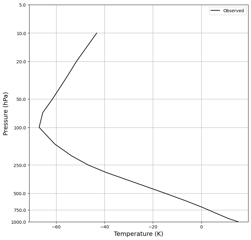
Observational estimate#
We start with the vertical thermal structure of the atmosphere in the reanalysis data.
#  This code is used just to create the skew-T plot of global, annual mean air temperature
%matplotlib inline
import numpy as np
import matplotlib.pyplot as plt
import xarray as xr
import climlab
from metpy.plots import SkewT

#plt.style.use('dark_background')

#ncep_url = "http://www.esrl.noaa.gov/psd/thredds/dodsC/Datasets/ncep.reanalysis.derived/"
ncep_url = "~/Desktop/ebooks/data"
ncep_air = xr.open_dataset( ncep_url + "/air.mon.1981-2010.ltm.nc", use_cftime=True)
#  Take global, annual average
coslat = np.cos(np.deg2rad(ncep_air.lat))
weight = coslat / coslat.mean(dim='lat')
Tglobal = (ncep_air.air * weight).mean(dim=('lat','lon','time'))

def zstar(lev):
    return -np.log(lev / climlab.constants.ps)

def plot_soundings(result_list, name_list, plot_obs=True, fixed_range=False):
    color_cycle=['r', 'g', 'b', 'y']
    # col is either a column model object or a list of column model objects
    #if isinstance(state_list, climlab.Process):
    #    # make a list with a single item
    #    collist = [collist]
    fig, ax = plt.subplots(figsize=(9,9))
    if plot_obs:
        ax.plot(Tglobal, zstar(Tglobal.level), color='k', label='Observed')
    for i, state in enumerate(result_list):
        Tatm = state['Tatm']
        lev = Tatm.domain.axes['lev'].points
        Ts = state['Ts']
        ax.plot(Tatm, zstar(lev), color=color_cycle[i], label=name_list[i])
        ax.plot(Ts, 0, 'o', markersize=12, color=color_cycle[i])
    #ax.invert_yaxis()
    yticks = np.array([1000., 750., 500., 250., 100., 50., 20., 10., 5.])
    ax.set_yticks(-np.log(yticks/1000.))
    ax.set_yticklabels(yticks)
    ax.set_xlabel('Temperature (K)', fontsize=14)
    ax.set_ylabel('Pressure (hPa)', fontsize=14)
    ax.grid()
    ax.legend()
    if fixed_range:
        ax.set_xlim([200, 300])
    ax.set_ylim(zstar(np.array([1000., 5.])))
    #ax2 = ax.twinx()

    return ax

plot_soundings([],[] )
<Axes: xlabel='Temperature (K)', ylabel='Pressure (hPa)'>
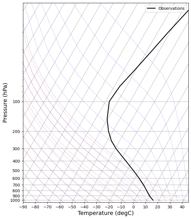
def make_skewT():
    fig = plt.figure(figsize=(9, 9))
    skew = SkewT(fig, rotation=30)
    skew.plot(Tglobal.level, Tglobal, color='k', linestyle='-', linewidth=2, label='Observations')
    skew.ax.set_ylim(1050, 10)
    skew.ax.set_xlim(-90, 45)
    # Add the relevant special lines
    skew.plot_dry_adiabats(linewidth=0.5)
    skew.plot_moist_adiabats(linewidth=0.5)
    #skew.plot_mixing_lines()
    skew.ax.legend()
    skew.ax.set_xlabel('Temperature (degC)', fontsize=14)
    skew.ax.set_ylabel('Pressure (hPa)', fontsize=14)
    return skew


skew = make_skewT()
Radiative equilibrium model#
Before we go into RCE model, we recap the important feature of considering only radiative process. We increase the complexity of radiative model, rather than just grey radiation, by using the rapid radiative transfer model in climlab.
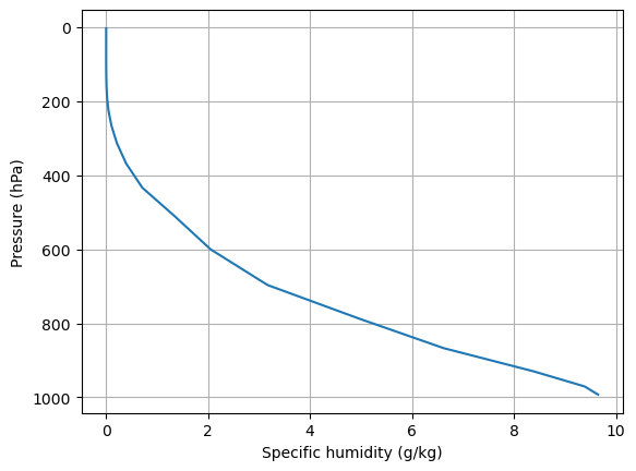
We load the water vapor profile from CESM control simulation.
# Load the model output as we have done before
#cesm_data_path = "/Users/yuchiaol_ntuas/Desktop/ebooks/local_ncu_climate_modelling/book_test2/docs/data/cpl_1850_f19.cam.h0.nc"
cesm_data_path = "~/Desktop/ebooks/data/cpl_1850_f19.cam.h0.nc"
atm_control = xr.open_dataset(cesm_data_path)

# The specific humidity is stored in the variable called Q in this dataset:
print(atm_control.Q)
print(atm_control.gw)


# Take global, annual average of the specific humidity
weight_factor = atm_control.gw / atm_control.gw.mean(dim='lat')

Qglobal = (atm_control.Q * weight_factor).mean(dim=('lat','lon','time'))
# Take a look at what we just calculated ... it should be one-dimensional (vertical levels)
print(Qglobal)

fig, ax = plt.subplots()
#  Multiply Qglobal by 1000 to put in units of grams water vapor per kg of air
ax.plot(Qglobal*1000., Qglobal.lev)
ax.invert_yaxis()
ax.set_ylabel('Pressure (hPa)')
ax.set_xlabel('Specific humidity (g/kg)')
ax.grid()
<xarray.DataArray 'Q' (time: 240, lev: 26, lat: 96, lon: 144)> Size: 345MB
[86261760 values with dtype=float32]
Coordinates:
  * lev      (lev) float64 208B 3.545 7.389 13.97 23.94 ... 929.6 970.6 992.6
  * time     (time) object 2kB 0001-02-01 00:00:00 ... 0021-01-01 00:00:00
  * lat      (lat) float64 768B -90.0 -88.11 -86.21 -84.32 ... 86.21 88.11 90.0
  * lon      (lon) float64 1kB 0.0 2.5 5.0 7.5 10.0 ... 350.0 352.5 355.0 357.5
Attributes:
    mdims:         1
    units:         kg/kg
    long_name:     Specific humidity
    cell_methods:  time: mean
<xarray.DataArray 'gw' (lat: 96)> Size: 768B
[96 values with dtype=float64]
Coordinates:
  * lat      (lat) float64 768B -90.0 -88.11 -86.21 -84.32 ... 86.21 88.11 90.0
Attributes:
    long_name:  gauss weights
<xarray.DataArray (lev: 26)> Size: 208B
array([2.16104904e-06, 2.15879387e-06, 2.15121262e-06, 2.13630949e-06,
       2.12163684e-06, 2.11168002e-06, 2.09396914e-06, 2.10589390e-06,
       2.42166155e-06, 3.12595653e-06, 5.01369691e-06, 9.60746488e-06,
       2.08907654e-05, 4.78823747e-05, 1.05492451e-04, 2.11889055e-04,
       3.94176751e-04, 7.10734458e-04, 1.34192099e-03, 2.05153261e-03,
       3.16844784e-03, 4.96883408e-03, 6.62218037e-03, 8.38350326e-03,
       9.38620899e-03, 9.65030544e-03])
Coordinates:
  * lev      (lev) float64 208B 3.545 7.389 13.97 23.94 ... 929.6 970.6 992.6
Now we construct a single column model.
#  Make a model on same vertical domain as the GCM
mystate = climlab.column_state(lev=Qglobal.lev, water_depth=2.5)
print(mystate)

radmodel = climlab.radiation.RRTMG(name='Radiation (all gases)',  # give our model a name!
                              state=mystate,   # give our model an initial condition!
                              specific_humidity=Qglobal.values,  # tell the model how much water vapor there is
                              albedo = 0.25,  # this the SURFACE shortwave albedo
                              timestep = climlab.constants.seconds_per_day,  # set the timestep to one day (measured in seconds)
                             )

print(radmodel)

#  Here's the state dictionary we already created
print('========================================')
print('=======radmodel.state=======')
print(radmodel.state)

#  Here are the pressure levels in hPa
print('========================================')
print('=======radmodel.lev=======')
print(radmodel.lev)

print('========================================')
print('=======radmodel.absorber_vmr=======')
print(radmodel.absorber_vmr)


#  specific humidity in kg/kg, on the same pressure axis
print('========================================')
print('=======radmodel.specific_humidity=======')
print(radmodel.specific_humidity)
AttrDict({'Ts': Field([288.]), 'Tatm': Field([200.  , 203.12, 206.24, 209.36, 212.48, 215.6 , 218.72, 221.84,
       224.96, 228.08, 231.2 , 234.32, 237.44, 240.56, 243.68, 246.8 ,
       249.92, 253.04, 256.16, 259.28, 262.4 , 265.52, 268.64, 271.76,
       274.88, 278.  ])})
climlab Process of type <class 'climlab.radiation.rrtm.rrtmg.RRTMG'>.
State variables and domain shapes:
  Ts: (1,)
  Tatm: (26,)
The subprocess tree:
Radiation (all gases): <class 'climlab.radiation.rrtm.rrtmg.RRTMG'>
   SW: <class 'climlab.radiation.rrtm.rrtmg_sw.RRTMG_SW'>
   LW: <class 'climlab.radiation.rrtm.rrtmg_lw.RRTMG_LW'>

========================================
=======radmodel.state=======
AttrDict({'Ts': Field([288.]), 'Tatm': Field([200.  , 203.12, 206.24, 209.36, 212.48, 215.6 , 218.72, 221.84,
       224.96, 228.08, 231.2 , 234.32, 237.44, 240.56, 243.68, 246.8 ,
       249.92, 253.04, 256.16, 259.28, 262.4 , 265.52, 268.64, 271.76,
       274.88, 278.  ])})
========================================
=======radmodel.lev=======
[  3.544638    7.3888135  13.967214   23.944625   37.23029    53.114605
  70.05915    85.439115  100.514695  118.250335  139.115395  163.66207
 192.539935  226.513265  266.481155  313.501265  368.81798   433.895225
 510.455255  600.5242    696.79629   787.70206   867.16076   929.648875
 970.55483   992.5561   ]
========================================
=======radmodel.absorber_vmr=======
{'CO2': 0.000348, 'CH4': 1.65e-06, 'N2O': 3.06e-07, 'O2': 0.21, 'CFC11': 0.0, 'CFC12': 0.0, 'CFC22': 0.0, 'CCL4': 0.0, 'O3': array([7.52507018e-06, 8.51545793e-06, 7.87041289e-06, 5.59601020e-06,
       3.46128454e-06, 2.02820936e-06, 1.13263102e-06, 7.30182697e-07,
       5.27326553e-07, 3.83940962e-07, 2.82227214e-07, 2.12188506e-07,
       1.62569291e-07, 1.17991442e-07, 8.23582543e-08, 6.25738219e-08,
       5.34457156e-08, 4.72688637e-08, 4.23614749e-08, 3.91392482e-08,
       3.56025264e-08, 3.12026770e-08, 2.73165152e-08, 2.47190016e-08,
       2.30518624e-08, 2.22005071e-08])}
========================================
=======radmodel.specific_humidity=======
[2.16104904e-06 2.15879387e-06 2.15121262e-06 2.13630949e-06
 2.12163684e-06 2.11168002e-06 2.09396914e-06 2.10589390e-06
 2.42166155e-06 3.12595653e-06 5.01369691e-06 9.60746488e-06
 2.08907654e-05 4.78823747e-05 1.05492451e-04 2.11889055e-04
 3.94176751e-04 7.10734458e-04 1.34192099e-03 2.05153261e-03
 3.16844784e-03 4.96883408e-03 6.62218037e-03 8.38350326e-03
 9.38620899e-03 9.65030544e-03]
Let’s have a look at the input parameters of RRTMG model, we can see a lot of parameters for cloud processes:
for item in radmodel.input:
    print(item)
specific_humidity
absorber_vmr
cldfrac
clwp
ciwp
r_liq
r_ice
emissivity
S0
insolation
coszen
eccentricity_factor
aldif
aldir
asdif
asdir
icld
irng
idrv
permuteseed_sw
permuteseed_lw
dyofyr
inflgsw
inflglw
iceflgsw
iceflglw
liqflgsw
liqflglw
tauc_sw
tauc_lw
ssac_sw
asmc_sw
fsfc_sw
tauaer_sw
ssaaer_sw
asmaer_sw
ecaer_sw
tauaer_lw
isolvar
indsolvar
bndsolvar
solcycfrac
Let’s integrate the model one timestep:
print('========================================')
print('=======radmodel.Ts=======')
print(radmodel.Ts)

print('========================================')
print('=======radmodel.Tatm=======')
print(radmodel.Tatm)

# a single step forward
radmodel.step_forward()

print('========================================')
print('=======radmodel.Ts=======')
print(radmodel.Ts)

climlab.to_xarray(radmodel.diagnostics)

climlab.to_xarray(radmodel.LW_flux_up)

print('========================================')
print('=======radmodel.ASR - radmodel.OLR=======')
print(radmodel.ASR - radmodel.OLR)
========================================
=======radmodel.Ts=======
[288.]
========================================
=======radmodel.Tatm=======
[200.   203.12 206.24 209.36 212.48 215.6  218.72 221.84 224.96 228.08
 231.2  234.32 237.44 240.56 243.68 246.8  249.92 253.04 256.16 259.28
 262.4  265.52 268.64 271.76 274.88 278.  ]
========================================
=======radmodel.Ts=======
[288.57727148]
========================================
=======radmodel.ASR - radmodel.OLR=======
[3.76767763]
The model does not reach equilibrium, right?
Now let’s integrate the model to equilibrium:
while np.abs(radmodel.ASR - radmodel.OLR) > 0.01:
    radmodel.step_forward()

#  Check the energy budget again
print('========================================')
print('=======radmodel.ASR - radmodel.OLR=======')
print(radmodel.ASR - radmodel.OLR)

def add_profile(skew, model, linestyle='-', color=None):
    line = skew.plot(model.lev, model.Tatm - climlab.constants.tempCtoK,
             label=model.name, linewidth=2)[0]
    skew.plot(1000, model.Ts - climlab.constants.tempCtoK, 'o',
              markersize=8, color=line.get_color())
    skew.ax.legend()

skew = make_skewT()
add_profile(skew, radmodel)
skew.ax.set_title('Pure radiative equilibrium', fontsize=18);
========================================
=======radmodel.ASR - radmodel.OLR=======
[0.00988074]
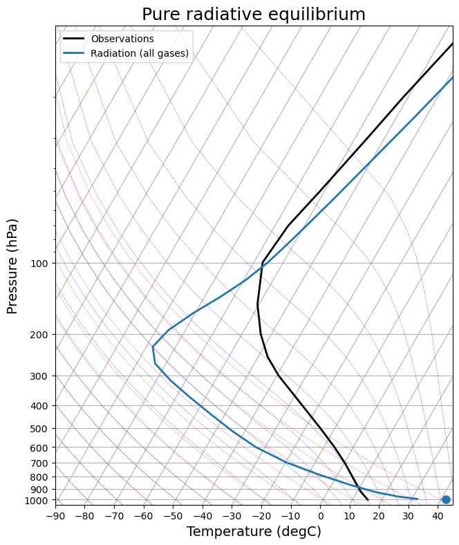
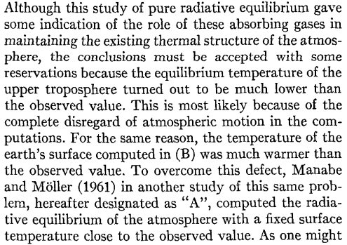
What do you think about the temperature profile compared to the observational one?
In Manabe’s 1964 paper:
Remove water vapor#
Let’s remove water vapor:
# Make an exact clone of our existing model
radmodel_noH2O = climlab.process_like(radmodel)
radmodel_noH2O.name = 'Radiation (no H2O)'

print('========================================')
print('=======radmodel_noH2O=======')
print(radmodel_noH2O)

#  Here is the water vapor profile we started with
print('========================================')
print('=======radmodel_noH2O.specific_humidity=======')
print(radmodel_noH2O.specific_humidity)

radmodel_noH2O.specific_humidity *= 0.

print('========================================')
print('=======radmodel_noH2O.specific_humidity=======')
print(radmodel_noH2O.specific_humidity)

#  it's useful to take a single step first before starting the while loop
#   because the diagnostics won't get updated
#  (and thus show the effects of removing water vapor)
#  until we take a step forward

radmodel_noH2O.step_forward()
while np.abs(radmodel_noH2O.ASR - radmodel_noH2O.OLR) > 0.01:
    radmodel_noH2O.step_forward()

print('========================================')
print('=======radmodel_noH2O.ASR - radmodel_noH2O.OLR=======')
print(radmodel_noH2O.ASR - radmodel_noH2O.OLR)

skew = make_skewT()
for model in [radmodel, radmodel_noH2O]:
    add_profile(skew, model)
========================================
=======radmodel_noH2O=======
climlab Process of type <class 'climlab.radiation.rrtm.rrtmg.RRTMG'>.
State variables and domain shapes:
  Ts: (1,)
  Tatm: (26,)
The subprocess tree:
Radiation (no H2O): <class 'climlab.radiation.rrtm.rrtmg.RRTMG'>
   SW: <class 'climlab.radiation.rrtm.rrtmg_sw.RRTMG_SW'>
   LW: <class 'climlab.radiation.rrtm.rrtmg_lw.RRTMG_LW'>

========================================
=======radmodel_noH2O.specific_humidity=======
[2.16104904e-06 2.15879387e-06 2.15121262e-06 2.13630949e-06
 2.12163684e-06 2.11168002e-06 2.09396914e-06 2.10589390e-06
 2.42166155e-06 3.12595653e-06 5.01369691e-06 9.60746488e-06
 2.08907654e-05 4.78823747e-05 1.05492451e-04 2.11889055e-04
 3.94176751e-04 7.10734458e-04 1.34192099e-03 2.05153261e-03
 3.16844784e-03 4.96883408e-03 6.62218037e-03 8.38350326e-03
 9.38620899e-03 9.65030544e-03]
========================================
=======radmodel_noH2O.specific_humidity=======
[0. 0. 0. 0. 0. 0. 0. 0. 0. 0. 0. 0. 0. 0. 0. 0. 0. 0. 0. 0. 0. 0. 0. 0.
 0. 0.]
========================================
=======radmodel_noH2O.ASR - radmodel_noH2O.OLR=======
[-0.00999903]
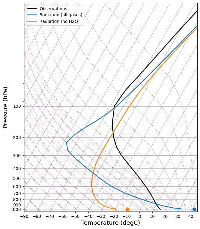
We can remove ozone and ozone and water vapor combined. Can you make the same plot?
Radiative convective equilibrium model#
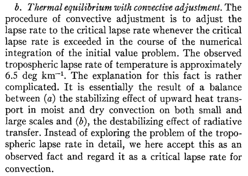
The idea is to copule the convective model to the radiative model. If the lapse rate exceeds the critical lapse rate, then an instantaneous adjustment will be performed to mix temperatures to the critical lapse rate while conserving the energy.
The crtical lapse is generally chosen to be 6.5 K / km. Let’s have a look at how Manabe discussed the critical lapse rate:
This is how we parameterize it and construct our RCE model in climlab:
#  Make a model on same vertical domain as the GCM
mystate = climlab.column_state(lev=Qglobal.lev, water_depth=2.5)

#  Build the radiation model -- just like we already did
rad = climlab.radiation.RRTMG(name='Radiation (net)',
                              state=mystate,
                              specific_humidity=Qglobal.values,
                              timestep = climlab.constants.seconds_per_day,
                              albedo = 0.25,  # surface albedo, tuned to give reasonable ASR for reference cloud-free model
                             )
#  Now create the convection model
conv = climlab.convection.ConvectiveAdjustment(name='Convection',
                                               state=mystate,
                                               adj_lapse_rate=6.5, # this is the key parameter! We'll discuss below
                                               timestep=rad.timestep,  # same timestep!
                                              )
#  Here is where we build the model by coupling together the two components
rcm = climlab.couple([rad, conv], name='Radiative-Convective Model')

print(rcm)
climlab Process of type <class 'climlab.process.time_dependent_process.TimeDependentProcess'>.
State variables and domain shapes:
  Ts: (1,)
  Tatm: (26,)
The subprocess tree:
Radiative-Convective Model: <class 'climlab.process.time_dependent_process.TimeDependentProcess'>
   Radiation (net): <class 'climlab.radiation.rrtm.rrtmg.RRTMG'>
      SW: <class 'climlab.radiation.rrtm.rrtmg_sw.RRTMG_SW'>
      LW: <class 'climlab.radiation.rrtm.rrtmg_lw.RRTMG_LW'>
   Convection: <class 'climlab.convection.convadj.ConvectiveAdjustment'>
#  Some imports needed to make and display animations
from IPython.display import HTML
from matplotlib import animation

def get_tendencies(model):
    '''Pack all the subprocess tendencies into xarray.Datasets
    and convert to units of K / day'''
    tendencies_atm = xr.Dataset()
    tendencies_sfc = xr.Dataset()
    for name, proc, top_proc in climlab.utils.walk.walk_processes(model, topname='Total', topdown=False):
        tendencies_atm[name] = proc.tendencies['Tatm'].to_xarray()
        tendencies_sfc[name] = proc.tendencies['Ts'].to_xarray()
    for tend in [tendencies_atm, tendencies_sfc]:
        #  convert to K / day
        tend *= climlab.constants.seconds_per_day
    return tendencies_atm, tendencies_sfc

def initial_figure(model):
    fig = plt.figure(figsize=(14,6))
    lines = []

    skew = SkewT(fig, subplot=(1,2,1), rotation=30)
    #  plot the observations
    skew.plot(Tglobal.level, Tglobal, color='black', linestyle='-', linewidth=2, label='Observations')
    lines.append(skew.plot(model.lev, model.Tatm - climlab.constants.tempCtoK,
              linestyle='-', linewidth=2, color='C0', label='RC model (all gases)')[0])
    skew.ax.legend()
    skew.ax.set_ylim(1050, 10)
    skew.ax.set_xlim(-60, 75)
    # Add the relevant special lines
    skew.plot_dry_adiabats(linewidth=0.5)
    skew.plot_moist_adiabats(linewidth=0.5)
    skew.ax.set_xlabel('Temperature ($^\circ$C)', fontsize=14)
    skew.ax.set_ylabel('Pressure (hPa)', fontsize=14)
    lines.append(skew.plot(1000, model.Ts - climlab.constants.tempCtoK, 'o',
                  markersize=8, color='C0', )[0])

    ax = fig.add_subplot(1,2,2, sharey=skew.ax)
    ax.set_ylim(1050, 10)
    ax.set_xlim(-8,8)
    ax.grid()
    ax.set_xlabel('Temperature tendency ($^\circ$C day$^{-1}$)', fontsize=14)

    color_cycle=['g','b','r','y','k']
    #color_cycle=['y', 'r', 'b', 'g', 'k']
    tendencies_atm, tendencies_sfc = get_tendencies(rcm)
    for i, name in enumerate(tendencies_atm.data_vars):
        lines.append(ax.plot(tendencies_atm[name], model.lev, label=name, color=color_cycle[i])[0])
    for i, name in enumerate(tendencies_sfc.data_vars):
        lines.append(ax.plot(tendencies_sfc[name], 1000, 'o', markersize=8, color=color_cycle[i])[0])
    ax.legend(loc='center right');
    lines.append(skew.ax.text(-100, 50, 'Day {}'.format(int(model.time['days_elapsed'])), fontsize=12))
    return fig, lines

def animate(day, model, lines):
    lines[0].set_xdata(np.array(model.Tatm)-climlab.constants.tempCtoK)
    lines[1].set_xdata(np.array(model.Ts)-climlab.constants.tempCtoK)
    #lines[2].set_xdata(np.array(model.q)*1E3)
    tendencies_atm, tendencies_sfc = get_tendencies(model)
    for i, name in enumerate(tendencies_atm.data_vars):
        lines[2+i].set_xdata(tendencies_atm[name])
    for i, name in enumerate(tendencies_sfc.data_vars):
        lines[2+5+i].set_xdata(tendencies_sfc[name])
    lines[-1].set_text('Day {}'.format(int(model.time['days_elapsed'])))
    # This is kind of a hack, but without it the initial frame doesn't appear
    if day != 0:
        model.step_forward()
    return lines
We use an isothermal initial condition:
#  Start from isothermal state
rcm.state.Tatm[:] = rcm.state.Ts

print('========================================')
print('=======rcm.state.Tatm=======')
print(rcm.state.Tatm)

#  Call the diagnostics once for initial plotting
rcm.compute_diagnostics()

#  Plot initial data
fig, lines = initial_figure(rcm)
========================================
=======rcm.state.Tatm=======
[288. 288. 288. 288. 288. 288. 288. 288. 288. 288. 288. 288. 288. 288.
 288. 288. 288. 288. 288. 288. 288. 288. 288. 288. 288. 288.]
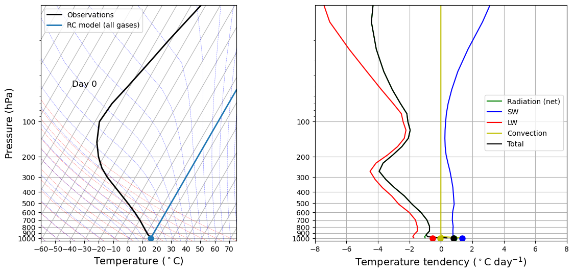
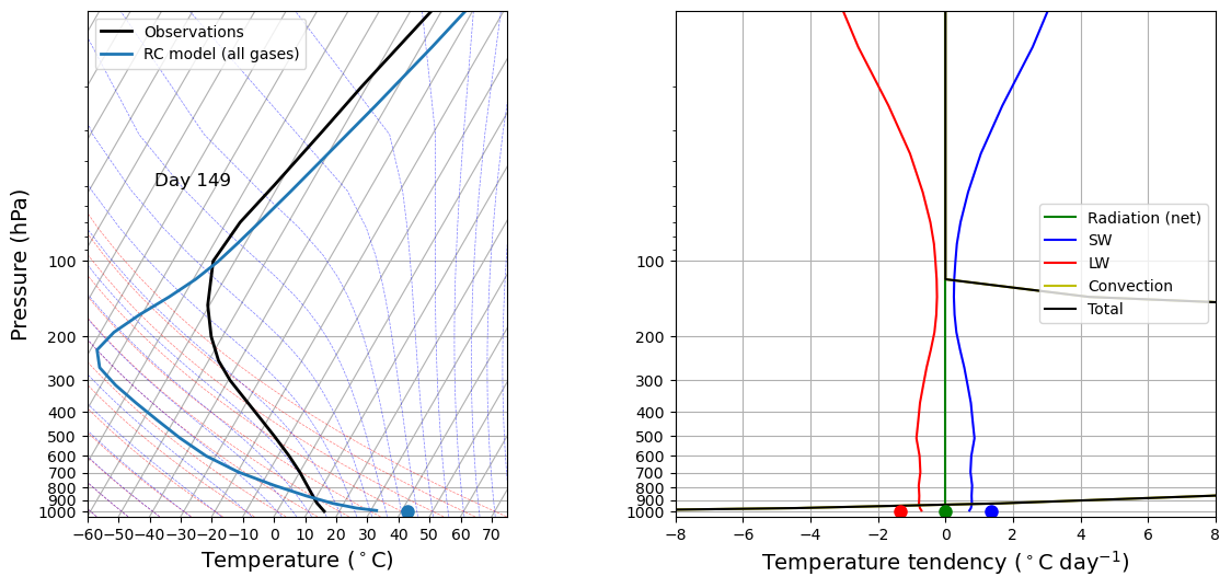
Below we follow Professor Brian Rose to create animations to illustrate the adjustment of RCE.
#  This is where we make a loop over many timesteps and create an animation in the notebook
ani = animation.FuncAnimation(fig, animate, 150, fargs=(rcm, lines))
HTML(ani.to_html5_video())
If we start from radiative equilibrium state:
#  Here we take JUST THE RADIATION COMPONENT of the full model and run it out to (near) equilibrium
#  This is just to get the initial condition for our animation
for n in range(1000):
    rcm.subprocess['Radiation (net)'].step_forward()
#  Call the diagnostics once for initial plotting
rcm.compute_diagnostics()
#  Plot initial data
fig, lines = initial_figure(rcm)
#  This is where we make a loop over many timesteps and create an animation in the notebook
ani = animation.FuncAnimation(fig, animate, 100, fargs=(rcm, lines))
HTML(ani.to_html5_video())
Note
Convection processes are fast compared to radiative processes.
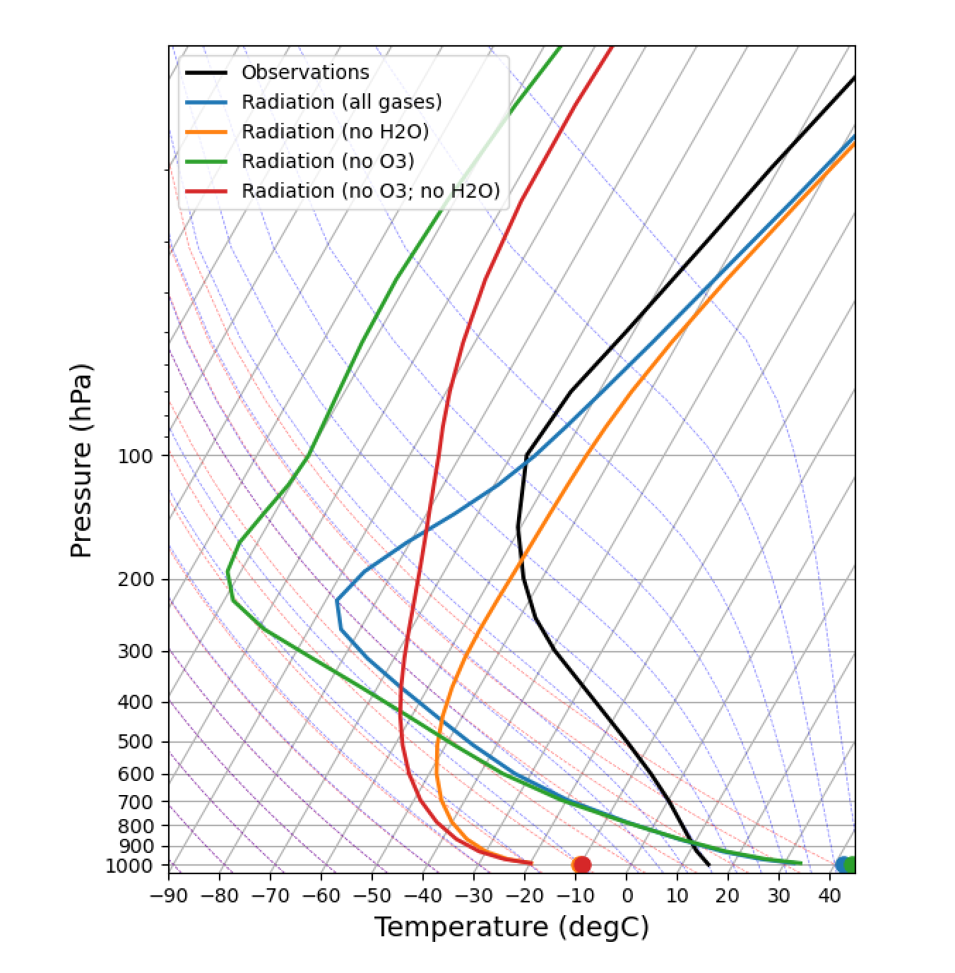
We now compare the results with those in radiative equilibrium.
#  Make a model on same vertical domain as the GCM
mystate = climlab.column_state(lev=Qglobal.lev, water_depth=2.5)

rad = climlab.radiation.RRTMG(name='all gases',
                              state=mystate,
                              specific_humidity=Qglobal.values,
                              timestep = climlab.constants.seconds_per_day,
                              albedo = 0.25,  # tuned to give reasonable ASR for reference cloud-free model
                             )

#  remove ozone
rad_noO3 = climlab.process_like(rad)
rad_noO3.absorber_vmr['O3'] *= 0.
rad_noO3.name = 'no O3'

#  remove water vapor
rad_noH2O = climlab.process_like(rad)
rad_noH2O.specific_humidity *= 0.
rad_noH2O.name = 'no H2O'

#  remove both
rad_noO3_noH2O = climlab.process_like(rad_noO3)
rad_noO3_noH2O.specific_humidity *= 0.
rad_noO3_noH2O.name = 'no O3, no H2O'

#  put all models together in a list
rad_models = [rad, rad_noO3, rad_noH2O, rad_noO3_noH2O]

rc_models = []
for r in rad_models:
    newrad = climlab.process_like(r)
    conv = climlab.convection.ConvectiveAdjustment(name='Convective Adjustment',
                                               state=newrad.state,
                                               adj_lapse_rate=6.5,  # the key parameter in the convection model!
                                               timestep=newrad.timestep,)
    rc = newrad + conv
    rc.name = newrad.name
    rc_models.append(rc)

for model in rad_models:
    for n in range(100):
        model.step_forward()
    while (np.abs(model.ASR-model.OLR)>0.01):
        model.step_forward()

for model in rc_models:
    for n in range(100):
        model.step_forward()
    while (np.abs(model.ASR-model.OLR)>0.01):
        model.step_forward()

skew = make_skewT()
for model in rad_models:
    add_profile(skew, model)
skew.ax.set_title('Pure radiative equilibrium', fontsize=18);

skew2 = make_skewT()
for model in rc_models:
    add_profile(skew2, model)
skew2.ax.set_title('Radiative-convective equilibrium', fontsize=18);
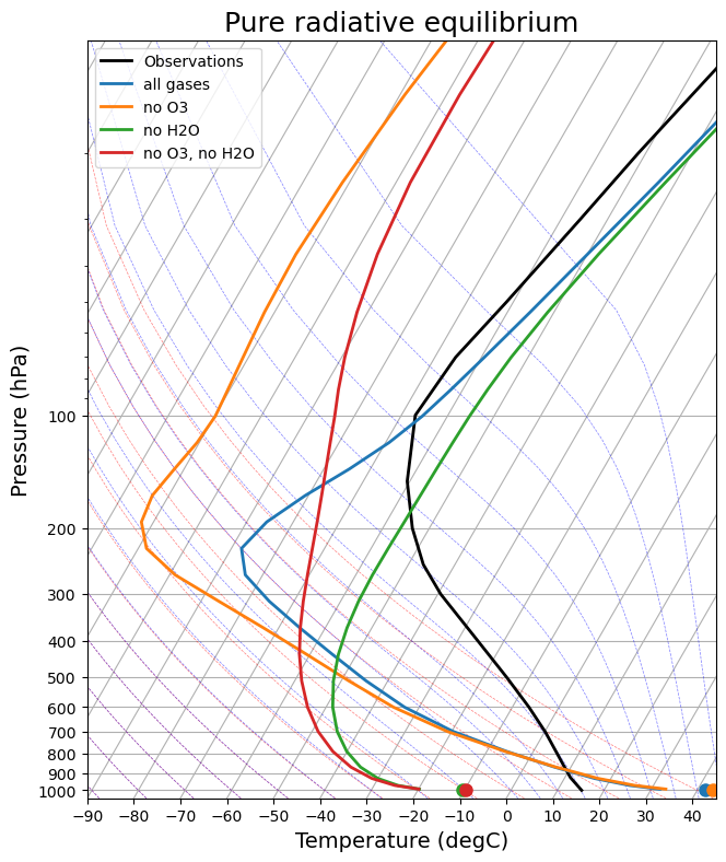
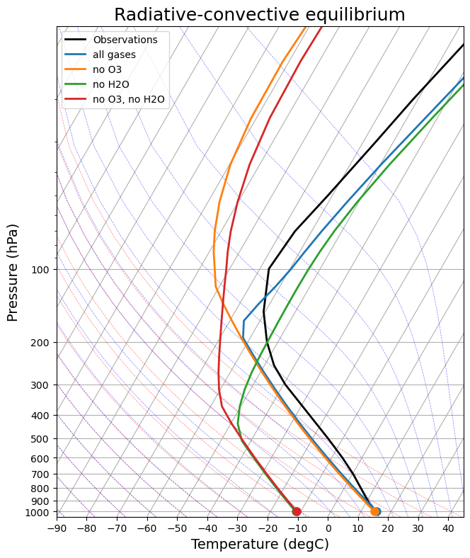
There are a lot to discuss. We could start with 1) the vertical structure, and 2) tropopause height.
Homework assignment 3 (due xxx)#
In the pure radiative model, can you remove the effect of ozone?
In the pure radiative model, can you remove the effects of ozone and water vapor?
In the RCE model, chosse an initial condition with temperature reaching radiative equilibrium.
In the RCE model, chosse an isothermal initial condition with temperature 360 K and 170 K. Can you plot the temperature evolution at surface, 800 hPa, 500 hPa, 200 hPa, and 100 hPa, with time?
Final project 4#
The key parameter ‘adj_lapse_rate’ determines the RCE equilibrium, but setting it as a constant may be somewhat idealized. Can you replace it with:
adj_lapse_rate = 9.8. This is the dry adiabatic lapse rate.
adj_lapse_rate = ‘pseudoadiabat’. This follows the blue moist adiabats on the skew-T diagrams.
more realistic lapse-rate from observations? For example from sounding?
Fig. 43 Credit to 中央大氣李恒安同學#
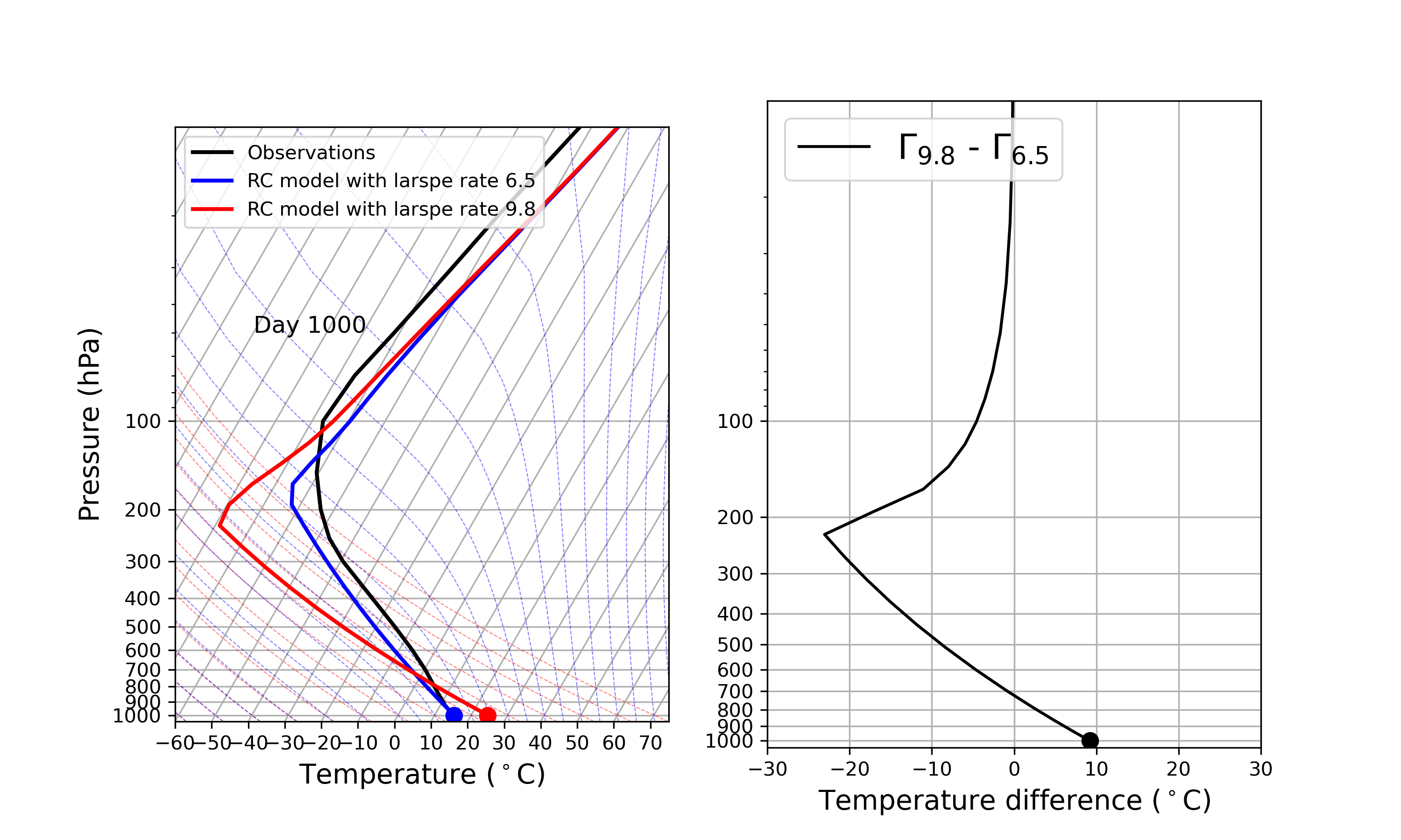
Fig. 44 Credit to 中央大氣何文樸同學#